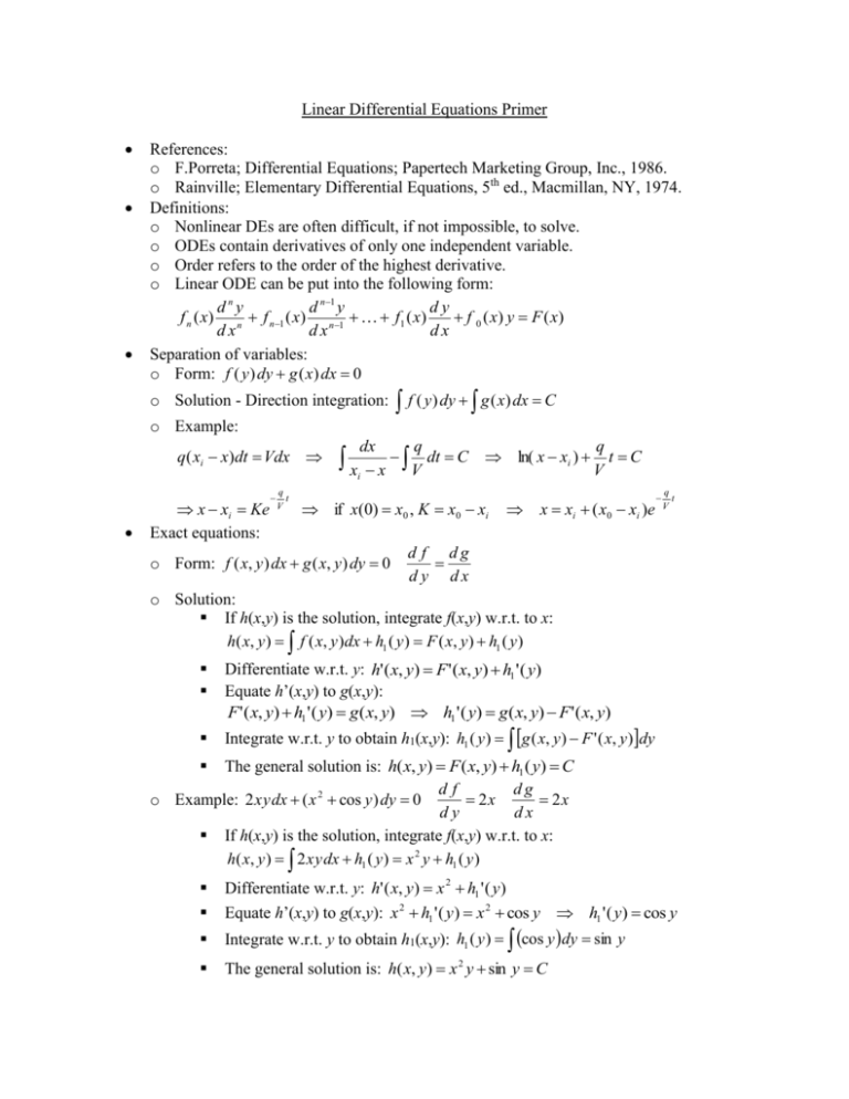
Linear Differential Equations Primer



References:
o F.Porreta; Differential Equations; Papertech Marketing Group, Inc., 1986.
o Rainville; Elementary Differential Equations, 5th ed., Macmillan, NY, 1974.
Definitions:
o Nonlinear DEs are often difficult, if not impossible, to solve.
o ODEs contain derivatives of only one independent variable.
o Order refers to the order of the highest derivative.
o Linear ODE can be put into the following form:
dny
d n1 y
dy
f n ( x) n  f n1 ( x) n1    f1 ( x)
 f 0 ( x) y  F ( x)
dx
dx
dx
Separation of variables:
o Form: f ( y ) dy  g ( x) dx  0
o Solution - Direction integration:
 f ( y) dy   g ( x) dx  C
o Example:
q( xi  x)dt  Vdx 

 x  xi  Ke
Exact equations:

q
t
V
dx
q
q
  dt  C  ln( x  xi )  t  C
V
V
i x
x
 if x(0)  x0 , K  x0  xi
o Form: f ( x, y ) dx  g ( x, y ) dy  0

x  xi  ( x0  xi )e

q
t
V
d f dg

dy dx
o Solution:
 If h(x,y) is the solution, integrate f(x,y) w.r.t. to x:
h( x, y )   f ( x, y )dx  h1 ( y )  F ( x, y )  h1 ( y )



Differentiate w.r.t. y: h' ( x, y)  F ' ( x, y)  h1 ' ( y)
Equate h’(x,y) to g(x,y):
F ' ( x, y)  h1 ' ( y)  g ( x, y)  h1 ' ( y)  g ( x, y)  F ' ( x, y)
Integrate w.r.t. y to obtain h1(x,y): h1 ( y )   g ( x, y )  F ' ( x, y )dy
The general solution is: h( x, y)  F ( x, y)  h1 ( y)  C
df
dg
 2x
 2x
o Example: 2 xy dx  ( x 2  cos y ) dy  0
dy
dx
 If h(x,y) is the solution, integrate f(x,y) w.r.t. to x:
h( x, y )   2 xy dx  h1 ( y )  x 2 y  h1 ( y )



Differentiate w.r.t. y: h' ( x, y)  x 2  h1 ' ( y)
Equate h’(x,y) to g(x,y): x 2  h1 ' ( y)  x 2  cos y  h1 ' ( y)  cos y

Integrate w.r.t. y to obtain h1(x,y): h1 ( y )   cos y  dy  sin y

The general solution is: h( x, y)  x 2 y  sin y  C

Homogeneous equations:
dy
 y
 f 
o Form:
dx
x
o Solution:
y

 Let u 
x
dy
du
ux
dx
dx

Substitute and separate u and x and then integrate:

Substitute u = y/x to obtain the general solution.

dx
du

C
x
f (u )  u
dy
dy y
y2
 y
 y  x2  y2 
  1 2  f  
dx
dx x
x
x
y
dy
du

ux
 f u   u  1  u 2
Let u 
x
dx
dx
Substitute and separate u and x and then integrate:
dx
du
2
 x   1  u 2  C  ln u  1  u  ln x  ln C
o Example: x




 u  1  u 2  Kx

 Substitute u = y/x to obtain the general solution: y  x 2  y 2  Kx 2
First order linear equations:
dy
 P( x) y  Q( x)
o Form:
dx
o Solution:
 Determine the integrating factor p: p  exp  P( x)dx


Substitute p into the following expression to obtain the general solution:
py   pQ( x)dx  C
o Example (Series RL circuit):



dI  R  V
  I 
dt  L 
L
I (0)  0
 R 
R 
Determine the integrating factor p: p  exp   dt   exp  t 
 L 
L 
Substitute p into the following expression to obtain the general solution:
 V 
R 
 R 
 V  L 
R 
exp  t  I     exp  t  dt  C     exp  t   C
L 
 L 
 L  R 
L 
 L 
I 


V
 R 
 C exp   t 
R
 L 
V
V
C  C  
R
R
V
 R 
The final solution: I  1  exp   t 
R
 L 
Apply initial condition: 0 

nth order linear homogeneous equations with constant coefficients:
o Form:
dny
d n1 y
dy
An n  An1 n1    A1  A0 y  0 An , An1 ,, A1 , A0 are constants.
dx
dx
dx
o Solution:
 Construct an auxiliary equation:
An r n  An1r n1    A1r  A0  0
 Solve the auxiliary equation:
 For each distinct real root (ra): ya  Ca exp( ra x)
 For each set of repeat (m times) real roots (rb):
 m1

yb  Cb1  Cb 2 x    Cbm x m1 exp( rb x)   Cbi x i 1  exp( rb x)
 i 1

 For each pair of Complex roots (a  jb):
yc  Cc sin bx  C 'c cos bx exp( ax)
 General solution: y = ya + yb + yc
th
n order linear nonhomogeneous equations with constant coefficients:
o Form:
dny
d n1 y
dy
An n  An1 n1    A1  A0 y  f ( x) An , An1 ,, A1 , A0 are constants.
dx
dx
dx
o Solution (Undetermined coefficients):
 Find the homogenous solution yh of the ODE. Do not apply the initial
conditions to determine the constants here.
 Select a general form of the particular solution yp.
 Substitute yp and its derivatives into the ODE.
 Equate coefficients of like terms and solve for the constants in yp.
 Apply initial condition to the general solution (y = yh + yp) to determine
the constants in yh.
 The undetermined coefficients method is usually cumbersome and seldom
used in practice.
th
n order linear nonhomogeneous equations with constant coefficients:
o Form:
dny
d n1 y
dy
An n  An1 n1    A1  A0 y  f ( x) An , An1 ,, A1 , A0 are constants.
dx
dx
dx
o Solution (Variation of parameters – 2nd order equations):
 Determine the homogeneous solution: yh(x) = C1u1(x) + C2u2(x)
 Assume: y(x) = v1(x) u1(x) + v2(x) u2(x)
 Set up equation (1): v1’(x) u1(x) + v2(x) u2’(x) = 0
 Set up equation (2): v1’(x) u1’(x) + v2’(x) u2’(x) = f(x)
 Solve the above equations to obtain v1’(x) and v2’(x).
 Integrate v1’(x) and v2’(x) to obtain v1(x) and v2(x), which yield the general
solution: y(x) = v1(x) u1(x) + v2(x) u2(x)
 The variation of parameters method is more powerful but it is still too
messy, especially for higher-order equations.





nth order linear nonhomogeneous equations with constant coefficients:
o Form:
dny
d n1 y
dy
An n  An1 n1    A1  A0 y  f ( x) An , An1 ,, A1 , A0 are constants.
dx
dx
dx
o Solution (Laplace transform):
 Transform the equation into the Laplace domain:
n 1
n2




An s nY ( s)   s n1k Y ( k ) (0)  An1 s n1Y ( s)   s n2k Y ( k ) (0)  
k 0
k 0




2
A2 s Y ( s)  sY (0)  Y ' (0)  A1 sY ( s)  Y (0)  A0Y ( s)  F ( s)
 Solve the algebraic equation in the s-domain for Y(s).
 Transform Y(s) back to the time domain to obtain the solution y(t).
Power series solution of 2nd order linear equations:
o Form:
y" p( x) y ' q( x) y  0
o Solution (near an ordinary point or a regular singular point): The process of
solving this type of equations is quite tedious and will not be discussed here.
However, solutions to several important equations are presented here.
o Example: Hypergeometric equations
 Form:
x(1  x) y"[c  (a  b  1) x] y '(ab) y  0
 Solution:
y1  F (a, b; c; x)



y 2  x1c F (a  1  c, b  1  c;2  c, x)

(a ) n (b) n x n
(c) n n!
n 1
where
F (a, b; c; x)  1  
and
(a) n 
(Hypergeom etric function)
 ( a  n)
(a )

( x)   e    x 1d
0
(n  1)  n!
o Example: Hermite equations
 Form:
y"2 xy'2 y  0
 Solution:
y  H n x  
1 
 2n
 
(1) k n!(2 x) n 2 k

k!(n  2k )!
k 0
  stands for greatest integer 
1
n
2
Hermite polynomial
1
n
2
o Example: Laguerre’s equations
 Form:
x y"[1  x] y 'n y  0
 Solution:
n
y1  Ln ( x)   (n) k 
k 0
n
 (1) k n! x k
xk



(k!) 2 k 0  (n  k )! (k!) 2
Laguerre polynomial
(n) k ( H nk  H n  2 H k ) x k  (1) n n!(k  1)! x k  n
y 2  Ln ( x) ln x  

(k!) 2
k  n!2
k 1
k 1
o Example: Bessel’s equations with non-integer index
 Form:
x 2 y" x y'( x 2  n 2 ) y  0 n  integer
 Solution:

(1) k x 2 k  n
J n ( x)   2 k  n
Bessel function of the first kind
k!(k  n  1)
k 0 2
y  AJ n ( x)  BJ n ( x)
o Example: Bessel’s equations with integer index
 Form:
x 2 y" x y'( x 2  n 2 ) y  0 n  integer
 Solution:
y1  J n ( x)
n
y2 
2
n 1
1
J n ( x)
(n  1)!
y3  y 2 ln x  x n
(1) k x 2 k  n
2k
k 1 2 (1  n) k k!
n 1

(1) k 1 ( H k n  H k  H n1 ) x 2 k n
2 2 k 1 (1  n) n1 (k  n)!k!
k n


y 4  J n ( x) ln x
(1) k 1 (n  1)! x 2 k n
2 2 k 1n (1  n) k k!
k 0
n 1

1  (1) k 1 ( H k  H k  n ) x 2 k  n
 2 2k n (k  n)!k!
2 k n
o Example: Legendre’s equations with integer index
 Form:
(1  x) 2 y"2 x y'n(n  1) y  0
 Solution: We are only interested in the non-logarithmic solution here.
1 x 

y1  Pn ( x)  F   n, n  1;1;
 Legendre polynomial
2 



PDEs:
o Form: DEs contain derivatives of more than one independent variable.
o Solution:
 Separate the variables
 Solve the individual ODEs
 Apply boundary and/or initial conditions to determine unknown
coefficients (Fourier series expansion technique is often used to match
discontinuities)
o Example (One-dimensional heat transfer equation):
u
 2u
 h 2 2 0  t , 0  x  c;
t
x
u t 0  f ( x) 0  x  c;
u t 0  0 x  0; u t 0  0 x  c;
 Let: u(x,t) = u1(x) u2(t)
 u1 ( x) u 2 ' (t )  h 2 u1 " ( x) u 2 (t ) 



Separate the variables:
u 2 ' (t )
u " ( x)
2 2
 
h
  h 2 1

u 2 (t ) arbitrary constant
u1 ( x)
u 2 ' (t )
 h 2 2
u 2 (t )


u1 " ( x)
  2
u1 ( x)



time equation
space equation
Solve the two equations separately and combine the solutions to obtain the
general solution:
u1  A cos( x)  B sin(  x) u2  exp( h 2 2 t )
 u  u1 u2  exp( h 2 2 t ) A cos( x)  B sin(  x)
Determine and from the boundary conditions:
u t 0  0 x  0; u t 0  0 x  c;
 A  0 and

u 2 ' (t )
u " ( x)
 h2 1
u 2 (t )
u1 ( x)
sin(  c)  0   
n
c
  n h  2   n  
 u n  Bn exp  
x
 t  sin 
  c    c 
Use Fourier series to match the initial condition and obtain the final
solution:
u t 0  f ( x) 0  x  c;
  n h  2 
 n 
u ( x, t )   Bn exp  
x
 t  sin 
 c 
n 1
  c  

Bn 
2 c
 n 
f ( x) sin 
x  dx

0
c
 c 
y
o Example (Two-dimensional Laplace equation):
 2V  2V

0
x 2 y 2
 Let: V(x,y) = Vx(x) Vy(y)
 Vx ( x) V y " ( y )  Vx " ( x) V y ( y )  0 


b
0
V0
0
0
a
Vy " ( y)
Vy ( y)

x
Vx " ( x)
0
Vx ( x)
Separate the variables:
Vy " ( y)
V " ( x)
 x
 2
  2
Vx ( x)
Vy ( y)
Solve the two equations separately and combine the solutions to obtain the
general solution:
Vx " ( x)
 2  Vx  C1 sin x  C2 cos x
Vx ( x)
Vy " ( y)

  2  V y  C3 sinh y  C4 cosh y
Vy ( y)
Determine coefficients from the boundary conditions:
Vx (0)  0  C 2  0 V y (0)  0  C 4  0 Vx (a)  0   

n
a
 n 
 n 
 Vn  An sin 
x  sinh 
y
 a 
 a 
Use Fourier series to match the initial condition and obtain the final
solution:


 m b   m 
Vm ( y  b)    Am sinh 
x   V0
 sin 
 a   a 
m 1 
 m b  2V0 a  m x 
 Am sinh 
sin 

 dx
a 0  a 
 a 
4V0


m b 
2V0

1  cos m    m sinh 
 Am 
a


 m b 

m sinh 

0
 a 

 n y    n 
 sinh  a   sin  a x 

 

 V ( x, y )  4V0  
n

b
n



n  odd 
 sinh  a  


m  odd
m  even