Programs for numerical vibrational wave functions in internal coordinates
Petr Bour
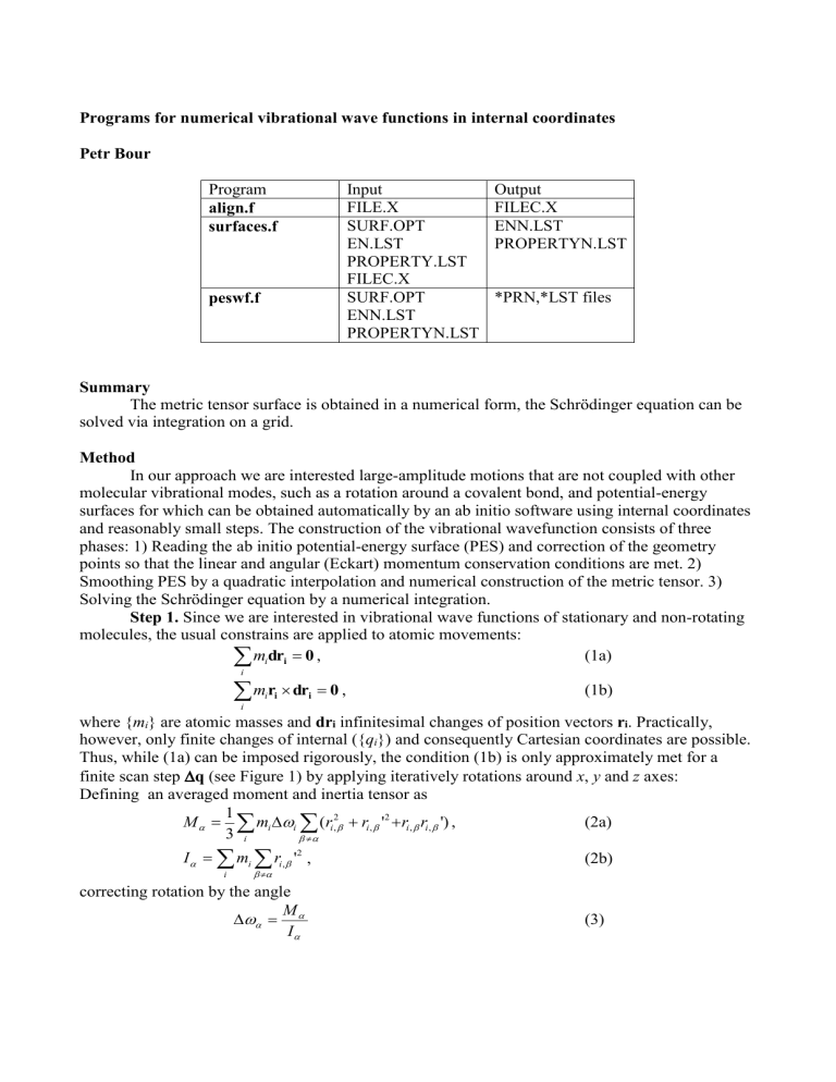
Program align.f surfaces.f peswf.f
Input
FILE.X
SURF.OPT
EN.LST
PROPERTY.LST
FILEC.X
SURF.OPT
ENN.LST
PROPERTYN.LST
Output
FILEC.X
ENN.LST
PROPERTYN.LST
*PRN,*LST files
Summary
The metric tensor surface is obtained in a numerical form, the Schrödinger equation can be solved via integration on a grid.
Method
In our approach we are interested large-amplitude motions that are not coupled with other molecular vibrational modes, such as a rotation around a covalent bond, and potential-energy surfaces for which can be obtained automatically by an ab initio software using internal coordinates and reasonably small steps. The construction of the vibrational wavefunction consists of three phases: 1) Reading the ab initio potential-energy surface (PES) and correction of the geometry points so that the linear and angular (Eckart) momentum conservation conditions are met. 2)
Smoothing PES by a quadratic interpolation and numerical construction of the metric tensor. 3)
Solving the Schrödinger equation by a numerical integration.
Step 1.
Since we are interested in vibrational wave functions of stationary and non-rotating molecules, the usual constrains are applied to atomic movements:
 m i dr i

0 , i i
 m i r i
 dr i

0 ,
(1a)
(1b) where { m i
} are atomic masses and dr i infinitesimal changes of position vectors r i
. Practically, however, only finite changes of internal ({ q i
}) and consequently Cartesian coordinates are possible.
Thus, while (1a) can be imposed rigorously, the condition (1b) is only approximately met for a finite scan step
 q (see Figure 1) by applying iteratively rotations around x , y and z axes:
Defining an averaged moment and inertia tensor as
M
I




1
3
 i m i
  i


 
  i m i
   r i ,

'
2
( r i
,
,
2

 r i ,

'
2  r i ,
 r i ,

' ) , (2a)
(2b) correcting rotation by the angle
 


M

I

(3)

is applied for

=x,y,z and repeated until convergence. In this way we obtain the Cartesian coordinates of all atoms as functions of the internal coordinates ( r i ,

 r i ,

( q
1
..
q
N
) ) for a standing non-rotating molecule.
Step 2.
In this step we have the possibility to smooth and resample the energy surface via a quadratic (spline) interpolation. More importantly, however, the metric tensor ( g ) and its inverse ( G
= g -1 ) are formed numerically using the coordinate dependence obtained at the previous step: g ij
( q
1
..
q
M
)

 
1
 
..
Nat m

  x , y , z
 r

 q i
,

 r

,

 q j
. (4) a T b
Step 3. The potential energy and metric tensor surfaces can be resampled again and smoothed either using polynomial or plane wave (cos, sin) functions, in order to obtain the final grid used in integration of the Schrödinger equation. The kinetic energy (T) integrals
 
1
2 a
, i
 j
G
1
4

 q i
G

1
2 G ij 
 q j
G
1
4 b (5a)
are transformed by integration per partes into
1
8
 j i ,
G ij


4
  b
 q j
 
 q i a

1
4
G

2

G
 q j

G
 q i
 b
 a

G

1


G q i
  b
 q j
 a


G
 q j
 b
 
 q i a


. (5b)
This is not necessary, but avoids estimation of the second wave function and G tensor derivatives.
Harmonic oscillator and plane wave (cos, sin) bases were used for the vibrational wavefunctions.
Time development of a wavepacket, from an initial

-function:

0
 
( q
10
..
q
M 0
)

N  i

1
 i
is the eigenfunction of H
1) Pure

: d i
0   i
( q
10
..
q
M 0
)
  j d c i
0 i j
 i
 j
( q
10
..
q
M 0
) ... and normalize
2) Temperature - determined
 d i
0   i
( q
10
..
q
M 0
) exp(
  i
/( kT )) ... and normalize
Propagate according to the Schrödinger equation d i
( t )
 d i
0 exp(
 i
 i t /  )

( t )
 i
N 

1 d i
0 exp(
 i
 i t /  )
 i
Calculation
Restriction: 1 and 2 dimension only.
1) On an equidistant grid, scan energy and geometry
2) Prepare FILE.X
with all geometries
3) Run allign to correct rotations/translations

4) Prepare EN.LST with all energies
5) Prepare SURF.OPT
with options

Example of the SURF.OPT option file:
NVAR number of variables
2 t FOR EACH: periodic boundary condition
48 number of grid points
0 360 min max
48 number of grid points for for H-calculation
15 10 26 number of basis functions for E G H
-1 0 0 kind of basis for E G H
10.0 75.0 200.0 freq, x0, red. mass (cm-1, any units, au=me) t FOR EACH: periodic boundary condition
48 number of grid points
0 360 min max
48 number of grid points for for H-calculation
15 10 26 number of basis functions for E G H
-1 0 0 kind of basis for E G H
10.0 150.0 200.0 freq, x0, red. mass (cm-1, any units, au=me)
STATES
4 1 2 3 4 states to plot
KINETIC
1 kind of the kinetic operator
PLANES
1 kind of plane waves
DIAG
1 kind of diagonalization
TEMPERATURE
273.15 temperature
Explanation: kind of basis for E G H
0 …. plane waves
1 … harmonics else .. quadratic fit kind of plane waves:
0: cos
1: cos and sin
2: sin
TEMP
T [298 K] temperature for probability plot

Advanced Options
TDEP ltime [false]
Continue with a propagation of the wavefunction
NTSTEP ntstep [10]
Number of time steps
DTSTEP dt [4.3]
Time increment
XT10 xt1 [0.0] x-coordinate of the initial packet position
XT20 xt2 [0.0] y-coordinate of the initial packet position

Examples
EN.LST
1.7 0.29225953
1.75 0.22554434
1.8 0.17188021
1.85 0.12894141
1.9 0.09481713
... first-coordinates, second – energies, relative, in au
ENN.LST
0 1.700000 0.292260 0.38451E-05
1 1.750000 0.225544 0.38451E-05
2 1.800000 0.171880 0.38451E-05
3 1.850000 0.128941 0.38451E-05
... first column- only number, second – fine coordinate, third 0 energy in au, fourth – metric tensor, for diatomic molecule =
4*0.527177^2/(M*1822.88)( M is atomic mass (g/mol))
0.38451E-05