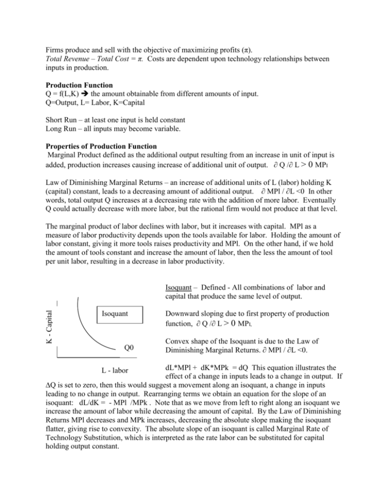
Firms produce and sell with the objective of maximizing profits (π).
Total Revenue – Total Cost = π. Costs are dependent upon technology relationships between
inputs in production.
Production Function
Q = f(L,K)  the amount obtainable from different amounts of input.
Q=Output, L= Labor, K=Capital
Short Run – at least one input is held constant
Long Run – all inputs may become variable.
Properties of Production Function
Marginal Product defined as the additional output resulting from an increase in unit of input is
added, production increases causing increase of additional unit of output. ∂ Q /∂ L > 0 MPI
Law of Diminishing Marginal Returns – an increase of additional units of L (labor) holding K
(capital) constant, leads to a decreasing amount of additional output. ∂ MPl / ∂L <0 In other
words, total output Q increases at a decreasing rate with the addition of more labor. Eventually
Q could actually decrease with more labor, but the rational firm would not produce at that level.
The marginal product of labor declines with labor, but it increases with capital. MPl as a
measure of labor productivity depends upon the tools available for labor. Holding the amount of
labor constant, giving it more tools raises productivity and MPl. On the other hand, if we hold
the amount of tools constant and increase the amount of labor, then the less the amount of tool
per unit labor, resulting in a decrease in labor productivity.
K - Capital
Isoquant – Defined - All combinations of labor and
capital that produce the same level of output.
Isoquant
Q0
Downward sloping due to first property of production
function, ∂ Q /∂ L > 0 MPI,
Convex shape of the Isoquant is due to the Law of
Diminishing Marginal Returns. ∂ MPl / ∂L <0.
dL*MPl + dK*MPk = dQ This equation illustrates the
effect of a change in inputs leads to a change in output. If
∆Q is set to zero, then this would suggest a movement along an isoquant, a change in inputs
leading to no change in output. Rearranging terms we obtain an equation for the slope of an
isoquant: dL/dK = - MPl /MPk . Note that as we move from left to right along an isoquant we
increase the amount of labor while decreasing the amount of capital. By the Law of Diminishing
Returns MPl decreases and MPk increases, decreasing the absolute slope making the isoquant
flatter, giving rise to convexity. The absolute slope of an isoquant is called Marginal Rate of
Technology Substitution, which is interpreted as the rate labor can be substituted for capital
holding output constant.
L - labor
.
Long Run Properties of Production:
2*K1
K - Capital
Returns to Scale
K1
Q1
Q0
L1
2*L1
L - labor
In the diagram to the left we double the
amount of inputs from L1, K1 to 2*L1
and 2*K1. Comparing the different
levels of output as measured by the two
isoquants, Q1 and Q2, defines the
following:
Increasing Returns Q1 >2Q 0
Doubling inputs more than doubles
output
Decreasing Returns Q1<2Q 0
Doubling inputs provides less than
double the output
Constant Returns
Q1=2Q 0
Doubling inputs doubles the output
*Assume Homogeniety- Slopes of
Isoquants along a capital labor ratio are the
same. Curvature of all isoquants is the
same.
K - Capital
K/L
Q1
MRTS is the same along a given K/L
Ratio, which allows the use of 1 isoquant
for representative purposes. Family of
isoquants is a map for technology.
Q0
L - labor
Profit maximization requires Cost Minimization
Isocost Line - all combinations of L and K which cost the same. Isocost derived from total
cost function.
Total Cost = (w * L) + (r * K); where w=wage rate, L=Labor, r=rental rate K=capital.
Rewriting this in terms of the variable K allows us to plot into our input space
diagram, K= (TC/r) – (w/r) L. This is the isocost curve whose properties are: the further
from the origin (out to the North East) the greater the total cost, and w/r, its slope in the wage
rental ratio, or the relative price of labor in terms of capital. With regards to the latter, the
steeper the isocost the more expensive labor is relative to capital. Of course the converse also
holds, the flatter the cheaper labor is relative to capital.
K - Capital
The closer the isocost line is to the origin,
the lower the Total Cost, e.g.,
TC0< TC1, note they have the same slope
(w/r). Comparing TC2 with either TC0 or
TC1 note TC2 is steeper thus illustrates a
relatively higher cost of capital.
TC1
K - Capital
TC2
TC0
K*
Cost Minimization
The rationale in cost minimization is
straightforward. If cost can be lowered then
L - labor
profits can be increased. Thus one condition
to maximize profits is to minimize costs.
With regards to our analysis that would
mean choosing the combination of labor and capital
that costs the least to produce a given amount of
output. For a given amount of output suggests that
we are restricted to a single isoquant. Finding the
least cost combination of labor and capital would
mean we need to be on the lowest feasible isocost.
That occurs at the tangency between isocost and
isoquant as in the diagram. L* and K* are the
lowest cost combination of L and K on Q0 given the
wage rental rate depicted as the slope of the isocost.
Q0
L*
L - labor
The least cost input bundle lies on the isocost line
tangent to the Isoquant. In other words the slopes of
the two are equal: -MPL/MPK = -w/r. Cross
multiplying leads to MPL/w = MPK/r, which is
interpreted as that the output per $ spent is equal
across all inputs. If this were not the case then the
firm could substitute the cheaper input for the more
expensive and thus lower costs.
How the firm responds to a change in input price.
A change in the price of an input, either labor or capital, will change the wage rental ratio and
consequently change the slope of the isocost curve. For example, if wages decrease, the isocost
line becomes flatter. Now the cost minimizing firm will need to seek a new set of inputs as a
K2
K1
K - capital
result of the price change. Seeking the new tangency between the isoquant and the new isocost
the firm will substitute labor for capital until their slopes are equal moving from L1, K1 down
and to the right to L2, K2.
w(1)/r
Q0
w(2)/r
L1
L2
L - labor