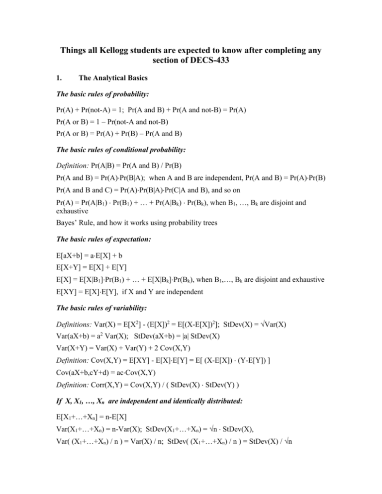
Things all Kellogg students are expected to know after completing any
section of DECS-433
1.
The Analytical Basics
The basic rules of probability:
Pr(A) + Pr(not-A) = 1; Pr(A and B) + Pr(A and not-B) = Pr(A)
Pr(A or B) = 1 – Pr(not-A and not-B)
Pr(A or B) = Pr(A) + Pr(B) – Pr(A and B)
The basic rules of conditional probability:
Definition: Pr(A|B) = Pr(A and B) / Pr(B)
Pr(A and B) = Pr(A)Pr(B|A); when A and B are independent, Pr(A and B) = Pr(A)Pr(B)
Pr(A and B and C) = Pr(A)Pr(B|A)Pr(C|A and B), and so on
Pr(A) = Pr(A|B1)  Pr(B1) + … + Pr(A|Bk)  Pr(Bk), when B1, …, Bk are disjoint and
exhaustive
Bayes’ Rule, and how it works using probability trees
The basic rules of expectation:
E[aX+b] = aE[X] + b
E[X+Y] = E[X] + E[Y]
E[X] = E[X|B1]Pr(B1) + … + E[X|Bk]Pr(Bk), when B1,…, Bk are disjoint and exhaustive
E[XY] = E[X]E[Y], if X and Y are independent
The basic rules of variability:
Definitions: Var(X) = E[X2] - (E[X])2 = E[(X-E[X])2]; StDev(X) = Var(X)
Var(aX+b) = a2 Var(X); StDev(aX+b) = |a| StDev(X)
Var(X+Y) = Var(X) + Var(Y) + 2 Cov(X,Y)
Definition: Cov(X,Y) = E[XY] - E[X]E[Y] = E[ (X-E[X])  (Y-E[Y]) ]
Cov(aX+b,cY+d) = acCov(X,Y)
Definition: Corr(X,Y) = Cov(X,Y) / ( StDev(X)  StDev(Y) )
If X, X1, …, Xn are independent and identically distributed:
E[X1+…+Xn] = n-E[X]
Var(X1+…+Xn) = n-Var(X); StDev(X1+…+Xn) = n  StDev(X),
Var( (X1+…+Xn) / n ) = Var(X) / n; StDev( (X1+…+Xn) / n ) = StDev(X) / n
Special distributions:
Binomial: If n independent trials each have probability p of being a “success,” then the
expected number of successes is np.
Geometric: If successive independent trials each have probability p of being a “success,”
then the expected number of trials up to and including the first success is 1/p.
Normal: Fully determined by  and . Appears in many settings due to the Central Limit
Theorem (stated intuitively). Sums, differences, and linear transformations of normallydistributed random variables are normally distributed.
Other skills:
Know how to construct and prune decision trees, determine value of information.
2.
Spreadsheet skills
Spreadsheet functions
=IF, =MAX, =MIN
=AND, =OR
=SUM, =COUNT, =AVERAGE, =PRODUCT
=SUMIF, =COUNTIF
=SUMPRODUCT
=COMBIN, =FACT
=LOOKUP
=BINOMDIST, =NORMDIST, =NORMINV, =TDIST, =TINV
=RAND, =RANDBETWEEN
=VAR, =STDEV
Spreadsheet tools
Data Table command
Solver
Simulation skills
=IF(RAND()<=p,1,0) simulates an event with probability p
=NORMINV(RAND(),mu,sigma) simulates a normally-distributed random variable
Familiarity with accumulating the results of spreadsheet simulation
3.
Key concepts to be discussed at some point
Understand, based on loose statement of Law of Large Numbers, why well-diversified
shareholders want managers to maximize expected returns.
Understand basic notions of risk aversion and utility maximization
Understand that the policy  that maximizes E[ f(X, ) ] (i.e., a “good” policy) is not
necessarily – indeed, is usually not – the policy  that maximizes f(E[X], ). In words:
The policy that would be optimal in the “expected” world is typically not the optimal
policy. This is a key justification for learning to work with simulations.
4.
Statistical skills and language
Understand confidence intervals for estimates of means and proportions (made using
simple random sampling)
Definition: “margin of error” = half-width of 95%-confidence interval
Can compute necessary sample size to achieve target margin of error (given appropriate
information, using simple random sampling)
Understand the concept underlying “degrees of freedom” (namely, that making multiple
estimates using the same sample – rather than with separate independent samples – ends
up making the estimates fit together a bit too well, and therefore requires an adjustment)
5.
Key applications
Can analyze portfolios of up to 3 stocks with dependent returns; understand idea behind
analysis of larger portfolios (without introducing matrix multiplication)
Single-period inventory problems: Understand the critical-fractile method.
Adverse selection: Have seen and understand how to address the phenomenon.