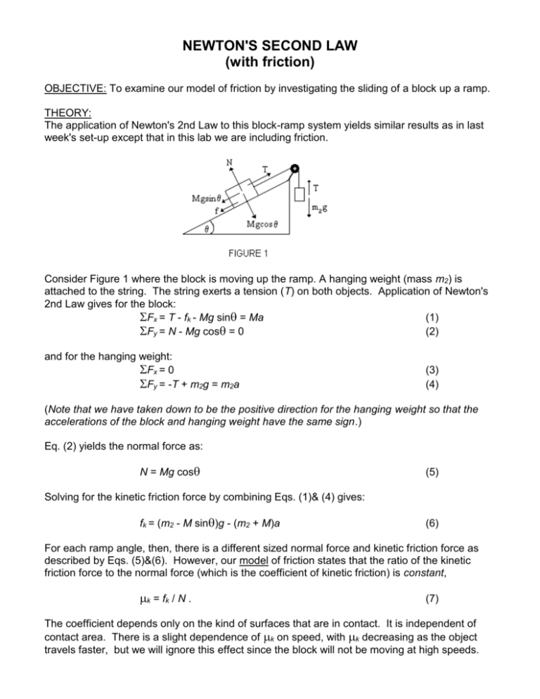
NEWTON'S SECOND LAW
(with friction)
OBJECTIVE: To examine our model of friction by investigating the sliding of a block up a ramp.
THEORY:
The application of Newton's 2nd Law to this block-ramp system yields similar results as in last
week's set-up except that in this lab we are including friction.
Consider Figure 1 where the block is moving up the ramp. A hanging weight (mass m2) is
attached to the string. The string exerts a tension (T) on both objects. Application of Newton's
2nd Law gives for the block:
Fx = T - fk - Mg sin = Ma
(1)
Fy = N - Mg cos = 0
(2)
and for the hanging weight:
Fx = 0
Fy = -T + m2g = m2a
(3)
(4)
(Note that we have taken down to be the positive direction for the hanging weight so that the
accelerations of the block and hanging weight have the same sign.)
Eq. (2) yields the normal force as:
N = Mg cos
(5)
Solving for the kinetic friction force by combining Eqs. (1)& (4) gives:
fk = (m2 - M sin)g - (m2 + M)a
(6)
For each ramp angle, then, there is a different sized normal force and kinetic friction force as
described by Eqs. (5)&(6). However, our model of friction states that the ratio of the kinetic
friction force to the normal force (which is the coefficient of kinetic friction) is constant,
k = fk / N .
(7)
The coefficient depends only on the kind of surfaces that are in contact. It is independent of
contact area. There is a slight dependence of k on speed, with k decreasing as the object
travels faster, but we will ignore this effect since the block will not be moving at high speeds.
Newton’s 2nd Law (with friction) 2
PROCEDURE:
1. (a) Weigh your block to determine its mass, M. (b) Raise the ramp to 25. (c) Place the
block on the ramp with its largest area touching the ramp and the string tied to the eyelet so that
the string is parallel to the ramp when placed over the pulley. (d) Hang a weight, m2, on the
string so that the block slides up the ramp a measured distance s. (The yellow marks on the
ramp are 80 cm apart.) Measure the time, t, for this motion. Select a weight so that t>1 s.
(e)Estimate the uncertainty in the time, t. (f) Record the value of m2.
1-1. Calculate the acceleration of the block using your values of s and t and the
equation of motion for constant acceleration, a = 2s / t2.
1-2. Calculate the uncertainty of the acceleration, a . From the previous equation for
the acceleration, this uncertainty is a = 2 a ( t /t )
1-3. Calculate the normal force in Newtons using Eq. (5).
1-4. Calculate the kinetic friction force in Newtons using Eq. (6).
1-5. Calculate the uncertainty in the friction force, fk. From Eq. (6), this uncertainty is
fk = (m2 + M) a
1-6. Calculate the coefficient of kinetic friction using Eq. (7).
1-7. Calculate the uncertainty of the coefficient, k. From Eq. (7), this uncertainty is
k = fk / N. Express your value of the coefficient as k  k.
2. We now see if the area of contact between the ramp and block makes a difference.
(a) Repeat Step 1, but this time place the block on its side. Attach the string to the other eyelet
so that the string remains parallel to the ramp. Use the same hanging weight.
1-1. Are the two coefficient of friction values the same when their respective
uncertainties are considered?
2-2. Is the observation made in 2-1 consistent with our model of friction?
3. We now see how a change in mass affects the results. (a) Reattach the string to the original
eyelet and place the block on the ramp in its original orientation. (b) Add 200 gm of mass to the
top of the block. Note that M is now the block's original mass plus the 200 gm. (c) Repeat Step
1. You may have to increase the hanging mass.
2-2. Is the normal force larger, smaller, or the same compared to when the block was
lighter? Does this agree with theory?
2-2. Is the kinetic friction force larger, smaller, or the same? Does this agree with
theory?
3-3. Is the coefficient of kinetic friction larger, smaller, or the same? Consider the
uncertainties of each value. Does this agree with our theoretical model?
4. We now see how the ramp angle affects the results. (a) Remove the extra 200 gm from the
block and measure the times for the block to travel the distance s for ramp angles of 35, 45,
and 50. You may have to adjust the hanging weight.
1-1. Calculate the acceleration and friction force values for each ramp angle.
4-2. Calculate the normal force values for each ramp angle. Is the normal force
constant? Does it increase or decrease as the ramp angle increases?
Newton’s 2nd Law (with friction) 3
4-3.
4-4.
4-5.
4-6.
Calculate the coefficients of friction and the uncertainties in the coefficients as you
did in Step 1.
Plot the calculated fk vs. N values. Include the other data points from Steps 1&3.
Also, include the point (0,0). Calculate the slope of the line. According to our
theoretical model, the slope is the coefficient of kinetic friction since fk = k N.
Record the value of k obtained from your line.
The inclusion of the point (0,0) on your plot will help you in determining the best
line. It is a valid point since if there is no normal force, there cannot be any
friction. It is necessary to add it because it is not practical to obtain normal force
values for this experimental set-up that are less than approximately 1.3 Newtons.
Why not? (Hint: see Eq. (5))
Compare this value of k from the best line to the other values of k obtained in
earlier runs. To do this, perform the following. For each of the runs, subtract the
uncertainty k from the k value. Put these values in one column in Excel. Now
add the uncertainty k to the k value for each run. Put these values in the
column immediately to the right of the first column. In the next column to the right,
put in the k values. For example, if the coefficient for one of the runs is 0.382 
0.031 then you would enter the data as shown for this run.
k - k k + k
0.351
0.413
k
0.382
Once the three columns are completed, highlight the data in the three columns.
Select the “Chart Wizard” and choose the “Stock” plots. Choose the first Stock
choice, which is labeled the High-Low-Close plot. Click on “Next”. Choose
“Series in Columns” in the Data Range Window. Click on “Next” and complete the
chart formatting. This should produce a plot that shows each coefficient with its
respective uncertainty represented by a vertical line. The horizontal axis should
show the run number. Be sure to label the vertical axis with “Coefficient of
Friction” and the horizontal axis with “Run”. Now draw a horizontal line (either
using the draw tool or a ruler and pen) whose coefficient value is equal to the k
from the best line in the first plot. Does this horizontal line intersect all of the
vertical lines? If so, then the k from the best line agrees well with the individual
values when the respective uncertainties are included.
REPORT:
1. There is a large amount of raw data and calculated data in this experiment. Be sure that you
organize it clearly in your report. A table or tables would be best for displaying your results.
2. Answer all of the questions posed in the procedure part. DO NOT SIMPLY NUMBER THE
QUESTIONS AND WRITE DOWN ANSWERS. WRITE COMPLETE SENTENCES IN YOUR
DISCUSSION THAT FULLY ADDRESS AND ANSWER THE QUESTIONS.
3. What can you conclude about our model for friction? Review your results carefully before
answering this question. Ask yourself if any discrepancies found can be fully explained by
experimental uncertainties or by assumptions made in the model.