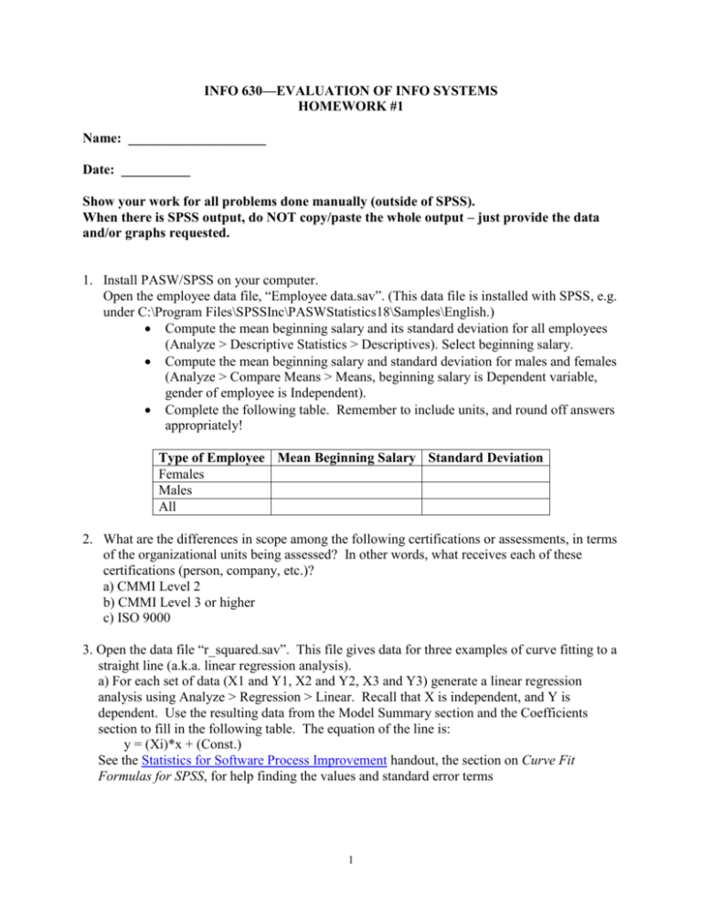
INFO 630—EVALUATION OF INFO SYSTEMS
HOMEWORK #1
Name: ____________________
Date: __________
Show your work for all problems done manually (outside of SPSS).
When there is SPSS output, do NOT copy/paste the whole output – just provide the data
and/or graphs requested.
1. Install PASW/SPSS on your computer.
Open the employee data file, “Employee data.sav”. (This data file is installed with SPSS, e.g.
under C:\Program Files\SPSSInc\PASWStatistics18\Samples\English.)
 Compute the mean beginning salary and its standard deviation for all employees
(Analyze > Descriptive Statistics > Descriptives). Select beginning salary.
 Compute the mean beginning salary and standard deviation for males and females
(Analyze > Compare Means > Means, beginning salary is Dependent variable,
gender of employee is Independent).
 Complete the following table. Remember to include units, and round off answers
appropriately!
Type of Employee Mean Beginning Salary Standard Deviation
Females
Males
All
2. What are the differences in scope among the following certifications or assessments, in terms
of the organizational units being assessed? In other words, what receives each of these
certifications (person, company, etc.)?
a) CMMI Level 2
b) CMMI Level 3 or higher
c) ISO 9000
3. Open the data file “r_squared.sav”. This file gives data for three examples of curve fitting to a
straight line (a.k.a. linear regression analysis).
a) For each set of data (X1 and Y1, X2 and Y2, X3 and Y3) generate a linear regression
analysis using Analyze > Regression > Linear. Recall that X is independent, and Y is
dependent. Use the resulting data from the Model Summary section and the Coefficients
section to fill in the following table. The equation of the line is:
y = (Xi)*x + (Const.)
See the Statistics for Software Process Improvement handout, the section on Curve Fit
Formulas for SPSS, for help finding the values and standard error terms
1
Case R Square Std Error Xi (B value +/- std error) Const. (B value +/- std error)
X1-Y1
X2-Y2
X3-Y3
b) Plot each case (Y1 vs X1, etc.) separately using Graphs > Legacy Dialogs > Scatter/Dot >
Simple Scatter (in older SPSS versions, use: Graphs > Scatter > Simple). Give each plot a
title and show it.
c) Describe the distribution of data for each case, and describe the resulting effect on R Square
and the standard error associated with the curve fit parameters.
4.
A uniform set of definitions and collection mechanisms for effort and size might be
advantageous across organizations. On the other hand, while advantageous, a uniform set of
definitions and collection mechanisms might not be feasible for software problems and
defects across organizations. Why?
5.
Before implementing a new software development environment, the productivity of your
team was 134 +/- 10 lines of code per staff month (LOC/month), where 10 LOC/month is
the standard error. After getting used to the new environment, the productivity was
measured at 177 +/- 13 LOC/month. To a 95% level of confidence, was there a statistically
significant improvement in productivity? Explain, and show your work!
(Hint: see the Statistical Q&A section in Statistics for Software Process Improvement.)
6. We want to know if there is a relationship between the productivity of programmers on a
project (in lines of code per month), and its average staffing level (computed by P=E/T where
E is the reported effort of the entire project in staff-months and T is the duration of the
project in calendar months). In other words, we are trying to find out what happens to
productivity for larger projects. To answer this, we have a data file of 187 projects from a
number of sources. These projects were written in a variety of languages and span the entire
spectrum of size and complexity.
a) Open the data file "project_productivity.sav". The variable “p_range” is the range of staffing
level, P, for the number of projects given by “freq” (for “frequency”). The average value of
productivity for those projects is given by “prdctvty”, which is expressed in LOC/staffmonth.
b) Determine the average productivity for the entire data set.
Use Analyze > Descriptive Statistics > Descriptives
Select prdctvty
Output: Write a sentence to describe the mean and standard deviation. Remember to include
units and round results appropriately!
c) Now weight the results by how many times each staffing level size category (p_range) was
reported.
Select Data > Weight Cases
Select "Weight cases by" and choose "freq"
Repeat step d to reassess the mean and standard deviation.
Output: Same as step b, noting that data were weighted by the frequency of each case.
2
d) Create a new variable called 'sequence' which has the average p_range for each row. So the
first value is (0+1)/2=0.5, the second is (1+2)/2=1.5, etc. For the last entry, use
sequence=150 for p_range >100.
e) Generate a scatter plot
Use Graphs > Legacy Dialogs > Scatter/Dot > Simple Scatter
Set Y = prdctvty and X = sequence
Output: your graph!
Note for copying SPSS graphs into MS Word: In SPSS, right click on the graph and copy it.
Go into Word, click once where you want it to go, and select Edit /
Paste Special. Select the Picture option and click Ok. Right click on the picture, and Format
Picture. Select the Layout tab, and make the picture is “In line with text.” Click Ok. Now the
image from SPSS is easy to resize and center as needed.
f) Generate a regression analysis of this data.
Use Analyze > Regression > Curve Estimation
Set Dependent Variable = prdctvty, and Independent Variable = sequence
Select Linear and Logarithmic Models
Check the box to have it “Display ANOVA table”
Output: Make a 3x3 table with the following data - Use "R Square" and "Standard Error" as
data columns, and Linear and Logarithmic for the rows. Fill it in!
g) Output: Based on their R2 values, which curve has the best fit?
Also note that the curve with the best fit should be visually closest to the Observed curve,
which is your input data. Is it a good fit?
h) Output: What does the best-fitting model tell you about the relationship between productivity
and project size as measured by productivity?
i) Output: What do you think are the major reasons that productivity behaves this way as a
function of team size?
7. This problem uses an excerpt from a Change Request (CR) database. CRs are problem
reports for an existing software system. We want to determine how long CRs took to be
completed (closed), based on their severity (criticality).
a) Open the data file "cr_closure.sav".
b) Define a new variable. Call it "clos_tim", and make its type Numeric.
Note that SPSS variable names formerly could only have eight characters. We won't use
them here, but labels may be attached to variables to describe them more fully.
c) Calculate the value of clos_tim
Use Transform > Compute Variable
Set the Target Variable as clos_tim (you have to type it in by hand)
For the Numeric Expression, use:
(closedat-opendate)/86400
[WHY? Dates are recorded in SPSS by the number of seconds. Hence the difference
between two dates is the number of seconds apart they are. To convert this to days,
divide by 60 sec/min*60 min/hr*24 hr/day, which is 86,400 sec/day.]
d) Now calculate the mean time to closure for CRs by their severity.
Use Analyze > Compare Means > Means
Select clos_tim as Dependent variable, and severity as Independent
3
Output: Fill in the table below. Be sure to identify the time unit for the mean and
standard deviation.
Time to Close for Change Requests
Change Request Type
Severity 1
Severity 2
Severity 3
All CRs
Mean
Here is the grading scale for the questions.
Problem
1
2
3a
3b
3c
4
5
6b
6c
6d
6e
6f
6g
6h
7d
TOTAL
Points
3
3
6
3 (1 per graph)
2
3
3
1
1
1
2
1
1
1
2
35 points
4
Std. Deviation