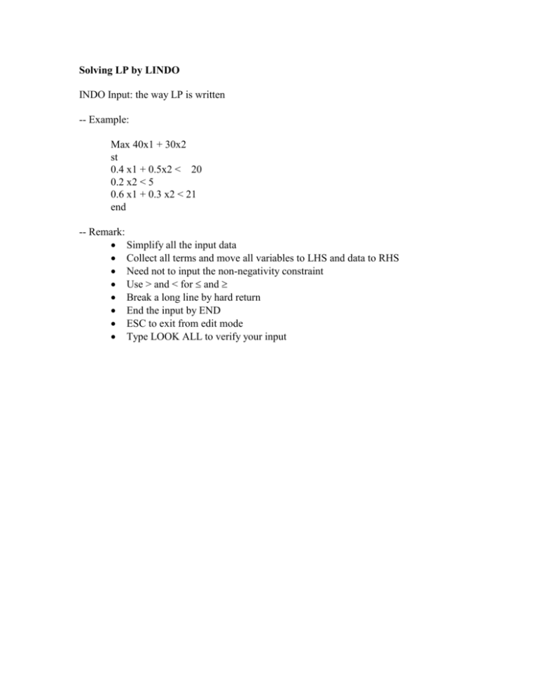
Solving LP by LINDO
INDO Input: the way LP is written
-- Example:
Max 40x1 + 30x2
st
0.4 x1 + 0.5x2 < 20
0.2 x2 < 5
0.6 x1 + 0.3 x2 < 21
end
-- Remark:
 Simplify all the input data
 Collect all terms and move all variables to LHS and data to RHS
 Need not to input the non-negativity constraint
 Use > and < for  and 
 Break a long line by hard return
 End the input by END
 ESC to exit from edit mode
 Type LOOK ALL to verify your input
LINDO Output
LP OPTIMUM FOUND AT STEP
2
OBJECTIVE FUNCTION VALUE
1)
VARIABLE
X1
X2
ROW
2)
3)
4)
1600.0000
VALUE
25.000000
20.000000
SLACK OR SURPLUS
.000000
1.000000
.000000
NO. ITERATIONS=
REDUCED COST
.000000
.000000
DUAL PRICES
33.333330
.000000
44.444440
2
RANGES IN WHICH THE BASIS IS UNCHANGED:
VARIABLE
X1
X2
ROW
2
3
4
OBJ COEFFICIENT RANGES
CURRENT
ALLOWABLE
ALLOWABLE
COEF
INCREASE
DECREASE
40.000000
20.000000
16.000000
30.000000
20.000000
10.000000
CURRENT
RHS
20.000000
5.000000
21.000000
RIGHTHAND SIDE RANGES
ALLOWABLE
ALLOWABLE
INCREASE
DECREASE
1.499999
6.000001
INFINITY
1.000000
9.000001
2.249999
Interpreting the LP Output:

Optimal OBJ:

Solution (Optimal Variable Value):

Reduced Cost of each variable:
Improvement needed in the objective coefficient (unit price, cost) for a current
zero variable (activity) to become positive.
or
Deterioration in objective value that occurs if the current zero variable is forced to
increase by one unit.
0 for a positive variable
+ for a zero variable

Slack or Surplus of each constraint:
Difference between LHS and RHS:
< constraint:
= resource available - resource used
> constraint:
= actual performance - requirement
Slack or Surplus = 0: binding constraint
* tight resource (for < constraint)
* requirement barely satisfied (for > constraint)
Slack or Surplus > 0: loose constraint
* abundant resource (for < constraint)
* requirement over fulfilled (for > constraint)

Dual Price of each constraint:
Improvement in the objective value if the RHS is increased by one unit.
* Value of additional resource
* Cost of more requirement



< constraint:
> constraint:
= constraint:
DP +
DP DP either sign
Dual Price  0 <==> Slack or Surplus = 0, binding constraint


Relationship Among Output data:

Variable value
0
+
vs.
Reduced Cost
+
0

Slack or Surplus
0
+
vs.
Dual Price
+ (< const), - (> const)
0
RHS Range:
The range that the RHS can change without changing the dual price of the binding
constraints and the current nonzero variables (status) in the solution.
Within the range:
* The marginal value of resource does not change (profit grows at constant
rate: DP).
* The structure of optimal solution (which product to produce) does not
change, however, the optimal solution (production quantities) will change
if the RHS of a binding constraint changes.

Obj. Coefficient Range:
The range that an objective coefficient can change without changing the current
optimal solution, however, both dual prices (of binding constraints) and reduce
costs (of non-zero variables) will change.
Questions based on the LP output of the RMC fuel and solvent example:
1.
2.
3.
4.
5.
How much material 2 has been used in the current production plan?
How much are you willing to pay an additional unit of material 1, 2, and 3?
Are you willing to pay $66.7 for additional 2 units of material 1?
Are you willing to sell 3 units of material 3 for $44.44 each unit?
Will you be interested in producing a new product, each of which sells for $50
and requires 0.6 unit of material 1, 0.4 unit of material 2 and 0.5 unit of
material 3?
6. If the price of fuel additive increases to $50 per unit, do you suggest change
the current production plan?
7. If the prices of fuel additive and solvent change to $45 and $35, respectively,
do you suggest change the current production plan?
8. How much are you willing to pay for 1 unit of Material 1, 2 units of Material
2, and 2 units of Material 3?
Solving LP by Microsoft EXCEL
Step 1. Organize the LP data in an Excel worksheet
Step 2. Establish the relationship between the Decision Variables and the Outputs
Step 3. Set Solver parameters (objective function and constraints)
 From menu bar, choose Tools and then Solver. A dialog box will show up.
 Set Target Cell to be the cell that contains the objective value.
 Specify Max or Min LP.
 Set Changing Cells to be cells that contain decision variables.
 Choose Add to input constraints in the dialog box. Repeat the process until all
constraints are inputted. Do not forget the nonnegativity constraints.
 When the above process is completed, choose OK. A summary of your inputs
will show up. Verify and make necessary changes.
Step 4. Solve the LP
 Choose Solve to solve the LP. A solution results dialog box will show up.
 In the Results section, select both Answer and Sensitivity.
 Choose OK to get the report sheets.
Interpreting the Excel solution
 Target Cell -- value of the objective function
 Adjustable Cells -- values of decision variables
 Status of each constraint and slack
 Reduced cost (for a zero decision variable) -- improvement needed in the
objective coefficient (unit price) for the variable (product) to be positive
(attractive, produced)
 Dual price (for a constraint) -- change (instead of improvement) of the
objective function value due to a unit increase of the RHS of the constraint.
 Ranges of objective function coefficients (so that the current optimal solution
remains unchanged)
 Ranges of RHSs of constraints (so that the current status of each constraint
(binding, not binding) and its dual price remain unchanged)
A Minimization LP Example for Output Interpretation
A 16-ounce can of dog food must contain protein, carbohydrate, and fat in at least the
following amounts: protein, 3 ounces; carbohydrate, 5 ounces; fat, 4 ounces. Four types
of gruel are to be blended together in various proportions to produce a least-cost can of
dog food satisfying these requirements. The contents and prices for 16 ounces of the gruel
are given below:
Contents
and price
Per 16 oz
of gruel
Gruel
Protein
Carbohydrate
Fat
Price ($)
1
3
7
5
4
2
5
4
6
6
3
2
2
6
3
4
3
8
2
2
Answer the following questions based on the LP output:
1. Interpret the optimal solution.
2. The dog food buyer is willing to pay $.6 more if you increase the protein content
by 0.5oz and keep the other contents unchanged. Do you want to accept the offer?
3. If the gruel 1 seller wants to offer you 20% discount on the product, will you be
interested in buying the gruel 1?
4. If the unit price of gruel 2 and 3 increase by $0.5 and that of gruel 4 decreases by
$0.5, do you want change the current dog food mix?
5. If you are allowed to change the dog food requirement by increasing the protein
by 0.5oz and decreasing the fat by 0.5oz, what would you recommend on the dog
food price?