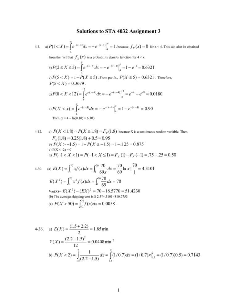
Solutions to STA 4032 Assignment 3

4.4.
a) P (1 

X )   e ( x4) dx   e( x4)  1 , because f X ( x)  0
4
for x < 4. This can also be obtained
4
from the fact that
f X (x)
is a probability density function for 4 < x.
5
b) P (2 
X  5)   e  ( x  4 ) dx   e  ( x  4 )  1  e 1  0.6321
5
4
4
c) P(5 
X )  1  P( X  5) . From part b., P( X  5)  0.6321 .
P(5  X )  0.3679 .
12
d) P(8 
X  12)   e  ( x  4) dx   e  ( x  4)
12
8
Therefore,
 e  4  e 8  0.0180
8
x
e) P ( X
 x)   e  ( x  4) dx   e  ( x  4 )
x
4
 1  e  ( x  4)  0.90 .
4
Then, x = 4  ln(0.10) = 6.303
4-12.
a)
P( X  1.8)  P( X  1.8)  FX (1.8)
FX (1.8)  0.25(1.8)  0.5  0.95
b) P( X  1.5)
c) P(X < -2) = 0
d)
 1  P( X  1.5)  1  .125  0.875
P(1  X  1)  P(1  X  1)  FX (1)  FX (1)  .75  .25  0.50
70
70
70
dx 
ln x |  4.3101
1
1 69 x
1
69
70
70 70
E ( X 2 )   x 2 f ( x)dx  
dx  70
1
1 69
2
2
Var(X)= E ( X )  ( EX )  70  18.5770  51.4230
70
4-30.
because X is a continuous random variable. Then,
(a)
E ( X )   xf ( x)dx  
70
(b) The average shipping cost is $ 2.5*4.3101=$10.7753
70
(c)
4-36.
P( X  50)   f ( x)dx  0.0058 .
50
(1.5  2.2)
 1.85 min
2
(2.2  1.5) 2
V (X ) 
 0.0408 min 2
12
2
2
1
2
dx   (1 / 0.7)dx  (1 / 0.7) x 1.5  (1 / 0.7)(0.5)  0.7143
b) P( X  2)  
(2.2  1.5)
1.5
1.5
a) E ( X ) 
1
x
c) F ( X ) 
x
1
x
1.5 (2.2  1.5) dy  1.5(1 / 0.7)dy  (1 / 0.7) y |1.5
for 1.5 < x < 2.2.
Therefore,
0,
x  1.5


F ( x)  (1 / 0.7) x  2.14, 1.5  x  2.2

1, 2.2  x

4-42.
a) P(1 < Z < 1) = P(Z < 1)  P(Z <- 1)
= 0.84134  0.15866
= 0.68268
b) P(2 < Z < 2) = P(Z < 2)  P(Z < -2)
= 0.97725-0.02275=0.9545
c) P(3 < Z < 3) = P(Z < 3)  P(Z < -3)
= 0.99865-0.00135=0.9973
d) P(Z > 3) = 1  P(Z < 3)
= 1-0.99865=0.00135
e) P(0 < Z < 1) = P(Z < 1)  P(Z < 0)
= 0.84134  0.5 = 0.34134
4-48.
a) P(X > x) = P Z 


x  5
 = 0.5.
4 
Therefore, x = 5.
x  5

 = 0.95.
4 

x  5

Therefore, P Z 
 = 0.05
4 

b) P(X > x) = P Z 
Therefore, x 4 5 = 1.64, and x = 1.56.
x5

 Z  1 = 0.2.
 4

c) P(x < X < 9) = P
Therefore, P(Z < 1)  P(Z < x 4 5 )= 0.2 where P(Z < 1) = 0.84134.
Thus P(Z < x 4 5 ) = 0.64134. Consequently, x 4 5 = 0.36 and x = 6.44.
x  5
35
Z
 = 0.95.
4 
 4
x  5
x  5


Therefore, P Z 
  P(Z < 0.5) = 0.95 and P Z 
  0.30854 = 0.95.
4 
4 


d) P(3 < X < x) = P
Consequently,
x  5

P Z 
 = 1.25854. Because a probability can not be greater than one, there is
4 

no solution for x. In fact, P(3 < X) = P(0.5 < Z) = 0.69146. Therefore, even if x is set
to infinity the probability requested cannot equal 0.95.
e) This part of the exercise was changed in Printing 3 from P( x < X < x) to
2
P( x < X  5 < x).
P( x < X  5 < x) = P(5  x < X < 5 + x) = P 5  x  5  Z  5  x  5 

4
4

= P  x  Z  x  = 0.99
4
 4
Therefore, x/4 = 2.58 and x = 10.32.
4-56.


a) P(X > 0.5) = P Z 
0.5  0.4 

0.05 
= P(Z > 2) = 1  0.97725
= 0.02275
0.5  0.4 
 0.4  0.4
Z

0.05 
 0.05
b) P(0.4 < X < 0.5) = P
= P(0 < Z < 2) = P(Z < 2)  P(Z < 0)
= 0.47725


c) P(X > x) = 0.90, then P Z 
x  0.4 
 = 0.90.
0.05 
x  0 .4
Therefore, 0.05 = 1.28 and x = 0.336.
3
4-66. a) P( X  4)  
i 0
e6 6i
 0.1512
i!
X
2
N (6, 6 )
P( X  4)  P( Z  466 )  P( Z  0.816)  0.2071
b) X is approximately
c) P(8  X  12)  P( 866  Z  1266 )  P(0.816  Z  2.45)  0.2001
4-68.
Let X denote the number of defective chips in the lot.
Then, E(X) = 1000(0.02) = 20, V(X) = 1000(0.02)(0.98) = 19.6.

a) P( X  25)  P Z 

25.5  20 
  P( Z  1.24)  1  P( Z  1.24)  0.107
19.6 
b)
P(20  X  30)  P(20.5  X  29.5)  P(
.5
Z
19.6
9.5
19.6
)  P(0.11  Z  2.15)
=P(Z<2.15)-P(Z<0.11)= 0.9842  0.5438  0.44
4-88.
Let X denote the distance between major cracks. Then, X is an exponential random
variable with   1 / E ( X )  0.2 cracks/mile.
3
a) P(X > 10) =


10
10
 0.2 x
 0.2 x
 0.2e dx   e
 e 2  0.1353
b) Let Y denote the number of cracks in 10 miles of highway. Because the distance
between cracks is exponential, Y is a Poisson random variable with   10(0.2)  2
cracks per 10 miles.
e 2 22
P(Y = 2) =
 0.2707
2!
c)  X  1/   5 miles.
d) P(12  X  15)  0.2e  0.2 x dx   e  0.2 x
15
15
12

12

e) P(X > 5) =  e  0.2 x
 e  2.4  e  3  0.0409
 e 1  0.3679 . By independence of the intervals in a Poisson
5
process, the answer is 0.36792  0.1353 . Alternatively, the answer is P(X > 10) =
e2  0.1353 . The probability does depend on whether or not the lengths of highway are
consecutive.
f) By the memoryless property, this answer is P(X > 10) = 0.1353 from part e).
4