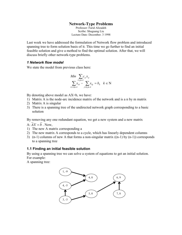
Network-Type Problems
Professor: Farid Alizadeh
Scribe: Shuguang Liu
Lecture Date: December. 3 1998
Last week we have addressed the formulation of Network flow problem and introduced
spanning tree to form solution basis of it. This time we go further to find an initial
feasible solution and give a method to find the optimal solution. After that, we will
discuss briefly other network-type problems.
1 Network flow model
We state the model from previous class here:
Min
c
(i,j)Α
x
i:(i,k)Α
ik

ij
xij
x
j:(k,j)Α
kj
 bk k  
By denoting above model as AX=b, we have:
1) Matrix A is the node-arc incidence matrix of the network and is a n by m matrix
2) Matrix A is singular
3) There is a spanning tree of the undirected network graph corresponding to a basic
solution
By removing any one redundant equation, we get a new system and a new matrix
~
~
A: AX  b . Now,
1) The new A matrix corresponding a
2) The new matrix A corresponds to a cycle, which has linearly dependent columns
3) (n-1) columns of new A that forms a non-singular matrix ((n-1) by (n-1)) corresponds
to a spanning tree
1.1 Finding an initial feasible solution
By using a spanning tree we can solve a system of equations to get an initial solution.
For example:
A spanning tree:
1, -9
4, 0
6, 9
5, 0
7, 8
4, -5
3, -3
Notes: The first number of two numbers in an ellipse denotes the number of nodes; the
second the demand of this nodes.
The corresponding system of equations:
 x14  9
x14  x 24  0
x32  x 24  5
 x35  x32  3
x35  x56  0
x56  x76  9
 x76  8
The easy way to solve this system is to first find equation with only one variable; that is
finding a leaf in the corresponding spanning tree.
We get the solution. But it is not feasible, because it violates the nonnegative constraints.
In fact, we need a procedure like phase 1 in the simplex method to get a feasible solution.
This procedure can be described shortly as follows:
Find a node receiving from all supplying nodes and sending to all other non-supply
nodes. If we can not find a qualified node, we can pick up a node and construct arcs
sending from all supplying nodes to this node or sending from this node to other non
supply nodes.
Then we solve the problem corresponding to this spanning tree. If this problem does not
have zero objective value (cost), then the original problem is infeasible. If it does, we can
obtain a feasible solution.
1.2 Using dual cost tree to find optimal solution
Dual problem of minimum network flow problem:
Max
b
k Ν
k
yk
y j  y i  cij (i,j)  Α
As to above system, we know that primal problem has n-1 nonbasic v
Suppose we have an initial primal flow solution:
1
7, 9
4
10, 9
6
10, 9
2
5, 5
12, 8
5
6, 8
7
3
Arcs on spanning tree
Arcs on Non-spanning tree
First number: cost; Second number: flow
The dual cost solution:
Set y1=0
1
3
y4=20
y6=27
7
4
10
6
10
2
y2=10
2
5
9
5
6
y5=21
3
3
12
7
y7=33
y3=15
Arcs on spanning tree
Arcs on Non-spanning tree
First number: cost; Second number: flow
From dual cost solution, check the optimality of primal problem:
We see that arc 14 does not satisfy optimality, so this arc should enter into the spanning
tree, which corresponds to a nonbasic variable. Now by adding arc 14 in primal flow tree,
we have a cycle. In this cycle we need to drop an arc to retain a spanning tree. Here we
back to primal flow tree:
1
t
4
9-t
9-t
2
Arcs on spanning tree
Arcs on Non-spanning tree
First number: cost; Second number: flow
From above, we set t=9. Then the whole primal flow tree:
1
-9
9
-5
9
4
0
6
2
5
8
8
5
7
3
-8
Arcs on spanning tree
Arcs on Non-spanning tree
First number: cost; Second number: flow
Dual cost tree:
Set y1=0
1
3
y4=3
y6=10
7
4
10
6
10
2
y2=10
5
6
3
2
9
3
12
5
y5=21
7
y7=33
y3=15
Arcs on spanning tree
Arcs on Non-spanning tree
First number: cost; Second number: flow
Check for optimality. All the arcs, which are off the spanning tree, satisfy the
inequalities. So, we find the optimal solution.
2. Shortest path problem
In this section, we seek the shortest paths from a source to all other nodes in a network.
h
18
a
a
h
9
c
c
6
6
12
S
s
d
2
9
d
g
g
f
f
13
b
b
12
6
e
10
e
17
A label-setting algorithm
Label notes starting from the source node by (node, distance).
Step 1: label source node:
S
S, 0
Step 2: separate labeled nodes from unlabeled nodes. And label node that has the shortest
distance from separated labeled notes set.
A, 6
a
b
b
6
S
S, 0
9
Keep doing step2 until all nodes have been labeled.
Step 3:
s, 6
18
a
6
S
S, 0
2
9
a, 8
b
c
c
Step 4:
S, 6
18
a
c
c
b,20
e
6
S
s
2
9
a, 8
b
12
Step 5:
S,6
18
a
a,24
c
6
S
S,0
d
2
9
a,8
d
g
g
f
f
h
h
e,26
g
f
f
13
b
12
6
b,20
10
e
17
Step 6:
S,6
18
a
a,24
6
9
c
6
S
S,0
d
2
9
a,8
d
13
b
12
6
b,20
e
17
Step 7:
h
S,6
18
a
a,24
6
h
9
c
6
12
S
S,0
c,30
2
9
a,8
d
e,26
g
f
f
c,33
h
13
b
12
6
b,20
e
17
Step 8:
S,6
18
a
a,24
6
9
c
6
12
S
S,0
c,30
2
9
a,8
d
e,26
g
f
f
c,33
h
13
b
12
6
b,20
10
e
17
Step 9:
S,6
18
a
a,24
6
9
c
6
12
S
S,0
c,30
2
9
a,8
e,26
g
e,37
f
13
b
12
6
b,20
10
e
17
Finally, we get the solution.
(s, a)=6
(s, b)=8
(s, c)=24
d
(s, d)=30
(s, e)=20
(s, f)=37
(s, g)=26
(s, h)=33
3 Maximum flow problem
Maximum flow problem is an another special type of network flow problem. This
problem can be stated as follows:
Suppose we have a network, which has one supplying node and one demanding node, and
the others are intermediate nodes. The objective is to push as much flow from the
supplying node to demanding node as possible. And the capacities of the arcs connecting
these nodes are not infinite (they are upper bounded).
c,24
b,6
S
c,30
t
a,8
d,20
Cts=-1
We can construct this problem by introducing a dummy arc from demanding node t to
supplying node s, and assuming cts negative (here it is set to -1). At the same time, we let
all cij=0 (the cost of transporting through arc ij), and let all the demands of all nodes to be
zero (bI=0).
Now since the only nonzero cost of the network is negative, we can transfer as much flow
as possible from demanding node t to supplying node s, in order to get maximum profit.
Now the model is as follows:
Max - xts
 xit   xtj  0
i:(i,k) Α
j:(k,j) Α
0  xij  u ij