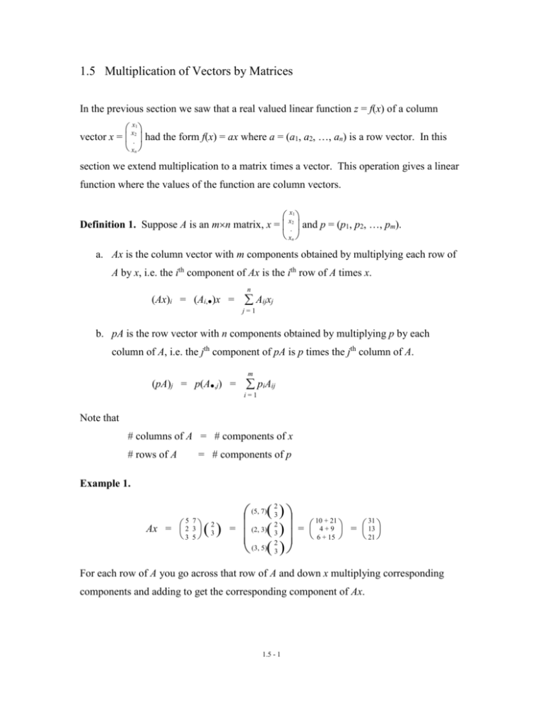
1.5 Multiplication of Vectors by Matrices
In the previous section we saw that a real valued linear function z = f(x) of a column
 xx21 
vector x =  .  had the form f(x) = ax where a = (a1, a2, …, an) is a row vector. In this
 xn 
section we extend multiplication to a matrix times a vector. This operation gives a linear
function where the values of the function are column vectors.
 xx21 
Definition 1. Suppose A is an mn matrix, x =  .  and p = (p1, p2, …, pm).
 xn 
a. Ax is the column vector with m components obtained by multiplying each row of
A by x, i.e. the ith component of Ax is the ith row of A times x.
n
(Ax)i = (Ai,●)x =  Aijxj
j=1
b. pA is the row vector with n components obtained by multiplying p by each
column of A, i.e. the jth component of pA is p times the jth column of A.
m
(pA)j = p(A●,j) =  piAij
i=1
Note that
# columns of A = # components of x
# rows of A
= # components of p
Example 1.
 (5, 7)( 3 ) 
 (2, 3)( 23 ) 
 (3, 5) 2 
 (3)
2
5 7
Ax =  2 3  ( 32 ) =
3 5
10 + 21
31
=  4 + 9  =  13 
 6 + 15 
 21 
For each row of A you go across that row of A and down x multiplying corresponding
components and adding to get the corresponding component of Ax.
1.5 - 1
5 7
pA = (2, 3, 5)  2 3  =
3 5
5
7


((2, 3, 5)  2  , (2, 3, 5)  3 )
3
5
= (10 + 6 + 15, 14 + 9 + 25) = (31, 48)
As with the product of a row vector and a column vector, the product of a matrix time a
vector is useful for describing linear functions.
Example 2. The three linear functions
 =
2x + y + z
 =
4x – 6y
 = - 2x + 7y + 2z
can be written either as
 
 2 1 1   x
 =  4 -6 0 y
-2 7 2z

or
w = Au
2 4 -2
(, , ) = (x, y, z)  1 - 6 7 
1 0 2
or
q = pB
or
 x
where u =  y ,
z
 
w =   ,

p = (x, y, z),
2 4 -2
A = 1 -6 7
1 0 2 
q = (, , )
2 4 -2
B = 1 -6 7
1 0 2
Similarly, the three linear equations
2x + y + z
=
4x – 6y
= -2
- 2x + 7y + 2z
=
5
9
can be written either as
 2 1 1   x
 5
 4 -6 0 y = -2
-2 7 2z
 9
or
1.5 - 2
Au = b
or
2 4 -2
(x, y, z)  1 - 6 7  = (5, - 2, 9)
1 0 2
or
pB = c
 5
where b =  - 2  and c = (5, - 2, 9).
 9
Example 3. In Example 4 in section 1.4 an electronics company made two types of circuit boards for
computers, namely ethernet cards and sound cards. Each of these boards requires a certain number of
resistors, capacitors and transistors as follows
resistors
capacitors
transistors
ethernet card
5
2
3
sound card
7
3
5
Let
e = # of ethernet cards the company makes in a certain day
s = # of sound card the company makes in a certain day
r = # of resistors needed to produce the e ethernet cards and s sound cards
c = # of capacitors needed to produce the e ethernet cards and s sound cards
t = # of transistors needed to produce the e ethernet cards and s sound cards
pr = price of a resistor
pc = price of a capacitor
pr = price of a transistor
pe = cost of all the resistors, inductors and transistors in an ethernet card
ps = cost of all the resistors, inductors and transistors in an sound card
Then we had the following linear functions.
e
r = 5e + 7s = (5, 7)  s  = (5, 7) x
e
c = 2e + 3s = (2, 3)  s  = (2, 3) x
e
t = 3e + 5s = (3, 5)  s  = (3, 5) x
5
5
pe = 5pr + 2pe + 3pt = (pr, pc, pt)  2  = p  2 
3
3
7
 
7
ps = 7pr + 3pe + 2pt = (pr, pc, pt)  3  = p  3 
2
2
where
e
x =  s 
p = (pr, pc, pt)
If we group r, c and t into a column vector y then we have
1.5 - 3
 (5, 7)  s  
 (2, 3)  e  
  es  
 (3, 5)  s  
e
y =
r
 5e + 7s 
 c  =  2e + 3s  =
t
 3e + 5s 
=
5 7
 2 3  x = Ax
3 5
where
5 7
A = 2 3
3 5
The point is that a set of linear equations can be represented compactly by a single vector matrix equation
y = Ax. Similarly, if we group pe and ps into a vector q then one has
5
7
q = (pe, ps) = (5pr + 2pe + 3pt, 7pr + 3pe + 2pt) = ((pr, pc, pt)  2 , (pr, pc, pt)  3  )
3
2
5
7


= (pr, pc, pt)  2 3  = pA
3 5
Identity Matrices. There is a special group of matrices called the identity matrices.
These are square matrices with the property that they have 1's on the main diagonal and
0's everywhere else. A square matrix is one where the number of rows and columns are
equal. The main diagonal of a matrix A are those entries whose row and column
subscripts are equal, i.e. the entries Aii for some i. The identity matrices are denoted by I.
Here are some identity matrices.
1
I =  0
1
I = 0
0
0
1
0 0
1 0
0 1
= the 22 identity matrix

 = the 33 identity matrix


I =
 10 01 00  00 


.
.
.

.


0 0 0  1
= the nn identity matrix
Thus
Iij =
1

0
if i = j
if i  j
These are called the identity matrices because they act like the number 1 for matrix
multiplication. If x is a column vector and p is a row vector then
1.5 - 4
Ix = x
pI = p
To see the first of these two relations, consider the ith component of Ix.
n
(Ix)i =  Iijxj
j=1
Since Iij = 0 unless j = i one has (Ix)i = Iiixi = xi. So Ix = x.
Another Way to Multiply a Vector by a Matrix. The following proposition gives
another way of viewing multiplication of a vector by a matrix.
Proposition 1.
a. Ax is the linear combination of the columns of A using the components of x as the
coefficients, i.e.
n
Ax = x1A●,1 + x2A●,2 +  + xnA●,n =  xjA●,j
j=1
b. pA is the linear combination of the rows of A using the components of p as the
coefficients, i.e.
pA = p1A1,● + p2A2,● +  + pmAm,● =
m
 piAi,●
p=1
Proof. To prove part a note that
n
n
n
j=1
j=1
j=1
(  xjA●,j)i =  xj(A●,j)i =  xjAij = (Ax)i
The proof of part b is similar. //
1.5 - 5
Example 3.
5 7 2
5
7
 10   21 
 31 
Ax =  2 3   3  = 2 2  + 3 3  =  4  +  9  =  13 
 21 
3 5
3
5
 6   15 
5 7
pA = (2, 3, 5)  2 3  = 2(5, 7) + 3(2, 3) + 5(3, 5)
3 5
= (10, 14) + (6, 9) + (15, 25) = (31, 48)
Algebraic Properties of Multiplication. The product of a vector and a matrix satisfies
many of the familiar algebraic properties of multiplication.
Proposition 2. If A and B are matrices, x and y are column vectors, p and q are row
vectors and t is a number then the following are true.
(A + B)x = Ax + Bx
A(x + y) = Ax + Ay
p(A + B) = pA + pB
(p + q)A = pA + qA
A(tx) = t(Ax)
(tA)x = t(Ax)
(tp)A = t(pA)
p(tA) = t(pA)
(Ax)T = xTAT
(pA)T = ATpT
p(Ax) = (pA)x
Proof. These are all easy to prove, so we leave the proof of most of them for an exercise.
We prove (Ax)T = xTAT and p(Ax) = p(Ax) as illustrations. To prove the first note that
((Ax)T)j = (Ax)j = (Aj,●)x = xT(Aj,●)T = xT((AT)●,j) = (xTAT)j. Note that we used the fact that
the jth column of AT is the same as the transpose of the jth row of A. To prove
p(Ax) = p(Ax) note that
n
n
n
n
m

m

m 
p(Ax) =  pi(Ax)i =  pi   Aijxj =    piAijxj =    bij


i=1
i = 1 j = 1
i = 1 j = 1
i = 1 j = 1 
m
m
m  n
m
n



 n 
(pA)x =  (pA)jxj =    piAij xj =    piAijxj =    bij
j = 1 i = 1 

j=1
j = 1i = 1 
j = 1i = 1
1.5 - 6
n
m  m  n 
where bij = piAijxj. In general    bij =    bij because in both case one is
i = 1 j = 1 
j = 1 i = 1 
summing bij over all combinations of i and j where i runs from 1 to n and j runs from one
to n. //
The following proposition is the analogue of Proposition 2 in section 1.4. It says that
multiplication by a matrix gives a linear function. It also says that all linear functions
z = T(x) where x and z are column vectors can be obtained by multiplication by a matrix.
Propostion 3. Let A be an mn matrix and let z = T(x) = Ax for any column vector
 x1 
x
x =  .2  with n components. Then T is linear, i.e. T(x + y) = T(x) + T(y) and T(tx) = tT(x)
 
 xn 
for any vectors x and y and number t. Furthermore, if z = T(x) is a linear function that
 x1 
 z1 
x
z
maps vectors x =  .2  to vectors z =  .2  with m components then there is an mn matrix
 
 
 xn 
 zm 
A such that T(x) = Ax.
Proof. The proof is very similar to the proof of Proposition 2 in section 1.4. First
suppose that z = T(x)= Ax for any x. Then T(x + y) = A(x + y) = Ax + Ay = T(x) + T(y)
where we used Proposition 2 for the second equality. Similarly T(tx) = A(tx) = t(Ax) =
tT(x) where we again used Proposition 2 for the second equality. So T is linear.
 x1 
x
Now suppose z = T(x) is linear. We can write x =  .2  = x1e1 + x2e2 + … + xnen where
 
 xn 
 0. 
ei =  1  is the vector such that every component is zero except the ith.
 0. 
0
0
So
T(x) = T(x1e1 + x2e2 + … + xnen) = x1T(e1) + x2T(e2) + … + xnT(en). If we let A be the
matrix such that A●,j = T(ej), then T(x) = A●,1x1 + A●,2x2 + … + A●,nxn = Ax which is what
we wanted to show. //
1.5 - 7