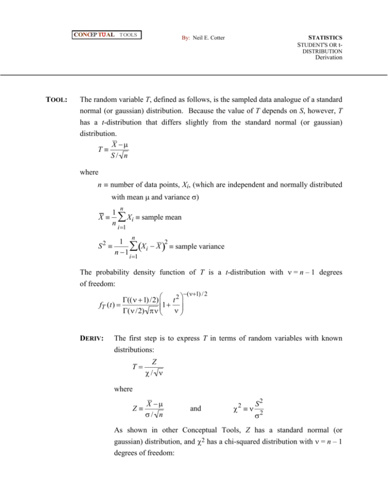
CONCEP TU AL TOOLS
STATISTICS
STUDENT'S OR t-
By: Neil E. Cotter
DISTRIBUTION
Derivation
TOOL:
The random variable T, defined as follows, is the sampled data analogue of a standard
normal (or gaussian) distribution. Because the value of T depends on S, however, T
has a t-distribution that differs slightly from the standard normal (or gaussian)
distribution.
X 
T
S/ n
where

n  number of data points, Xi, (which are independent and normally distributed
with mean  and variance )
X
n
1
 Xi  sample mean
n
i1

n
1
2
S 
X i  X   sample variance


n 1
2
i1
The probability density function of T is a t-distribution with  = n – 1 degrees
 of freedom:
(1) / 2
((  1) /2)  t 2 
1 
fT (t) 

( /2)  
  

DERIV:
The first step is to express T in terms of random variables with known
distributions:
T
Z
/ 
where

Z
X 
/ n
and
S2
2   2

As shown in other Conceptual Tools, Z has a standard normal (or
gaussian) distribution, and 2 has a chi-squared distribution with  = n – 1


degrees of freedom:
CONCEP TU AL TOOLS
STATISTICS
STUDENT'S OR t-
By: Neil E. Cotter
DISTRIBUTION
Derivation (cont.)
1 z 2 / 2
e
2
f Z (z) 

1
x ( / 2)1ex / 2
  / 2
f 2 (x)  2 ( /2)


0


x 0
x 0
As shown in another tool, Z and 2 are also independent. This allows us
to write the joint distribution of Z and 2 as the product of the respective
probability density functions for Z and 2:
 1 z 2 / 2
1
e
x ( / 2)1ex / 2


/
2
2 ( /2)
f (z, x)   2

0

x 0
x 0
To find the probability density for T, we consider the cumulative
distribution for T and take its derivative:
fT (t) 
NOTE:

d
d
d  
FT (t)  P(T  t) 
  z
dt
dt
dt  x /

t
f (z, x)dxdz
We treat the case of t > 0. We have t in the lower limit in this
case because larger values of x give smaller values of t. For the
case of t < 0, we would integrate from –∞ to t.
We move the derivative inside the outer integral and write the lower limit
in terms of the x more clearly:

fT (t) 

 d
 dt




x z
2
t2


f (z, x)dxdz


The chain rule yields an interpretation of the derivative of the integral:
d 
d 
dx
f (z, x)dx 
f (z, x)dx 


2
2
dt x z
dx x z
dt
2
2

t
or

t
CONCEP TU AL TOOLS
STATISTICS
STUDENT'S OR t-
By: Neil E. Cotter
DISTRIBUTION
Derivation (cont.)
d 
2z 2
2
f
(z,
x)dx


f
(z,
x)



x z
dt x z 2
t3
t2
2
t
Making this substitution, we have the following expression:

2z 2
2
fT (t) 
f (z, x) x z   3 dz

2
t


t
Now we use the expression for f(z, x), assuming t > 0:
z 2 

(
/
2)1




z 2 
 2 / 2
1 z 2 / 2
1
t 



e
 2 

f (z, x) x z 2   2 e
 /2
2
(
/2)
t



t2

0

NOTE:

z0
z0
We have the condition that z > 0 because the definition of T
requires Z > 0 to achieve T > 0. (X and X are always
positive.)
Incorporating the constraint on z into the lower limit of the outer integral

yields the following expression:
 2 
z
/ 2
2 ( / 2)1 



2
 1
1
z
2z 2
t 2 
z / 2



fT (t)  
e
e
 3 dz
 
0 2
2  / 2 ( /2)  t 2 
t
It is helpful to define a term for the constants:
k 2

1
1
1
1
   ( / 2)1 
 / 2

/
2
(1)
/
2
2 2 ( /2)
2
( /2)
Using this new term, we have the following expression:

fT (t)  k 
or

z 2 
(
/
2)1



2
 2 / 2z 2 1
 z 2 / 2z 
t 



e
e
 2 

 2 
t dz
0
t 
t 
CONCEP TU AL TOOLS
STATISTICS
STUDENT'S OR t-
By: Neil E. Cotter
DISTRIBUTION
Derivation (cont.)
fT (t)  k 

  
z 2 1 / 2  2  / 2
2

z
1
e  t  
 2 
 t dz
0
t
 
We define the following variable that allows us to use a convenient change
of variables:

zt  z 1 2
t
We have the following relationships for the change of variables:
dz t


 dz , z  0  zt  0 , z   zt 
1 2
t

and

2 1

zt2
1
2 1
21 1
2 1 t 

  zt 2
 zt
 zt  1 

t 2 1  t 2
t 
t2
 v 
1
2
t
v

z2
In terms of zt we have the following integral expression:

fT (t)  k 
 z t2 / 2
e
0
 t 2  / 2
 / 2
2  /2
zt
 1 


 
1

dzt
1
t2

or


fT (t)  k
 t 2 (1) / 2  2
z t / 2 2  / 2

1
e
zt
dzt

  
0


(1) / 2

We change variables again in order to make the integrand have the form of
a chi-squared distribution:
w  zt2
We have the following relationships for the change of variables:

CONCEP TU AL TOOLS
STATISTICS
STUDENT'S OR t-
By: Neil E. Cotter
DISTRIBUTION
Derivation (cont.)
dw
dw

 dzt , zt  0  w  0, zt   w 
2zt 2 w
In terms of w we have the following integral expression:



(1) / 2
2 


dw
(1) / 2 t 
fT (t)  k
 0 w  / 2ew / 2 2 w
1  


By moving appropriate constants inside the integral, we obtain the integral
of an entire chi-squared distribution with  + 1 degrees of freedom. In

other words the probability represented by the following integral must
equal unity:

0

1
2
(1) / 2
((  1) /2)
w ((1) / 2)1ew / 2 dw  1
It follows that we have the following expression for the probability density
function for T:
fT (t)  k2
(1) / 2
((  1) /2)
 t 2 (1) / 2
1  



(1) / 2
Simplification of the constants yields the final result:


(1) / 2
((  1) /2)  t 2 
1 
fT (t) 

( /2)  
  