AP STATISTICS: INFERENCE ANSWER KEY
1. For this problem, I will use a 1-sample z test. (I am assuming the population standard deviation is 12 grams) I am interested in the parameter

, the mean weight of an apple.
H
0
H a
:

= 120 The true mean weight of apples from the company is 120 grams.
:
 
120 The true mean weight of apples from the company is not 120 grams.
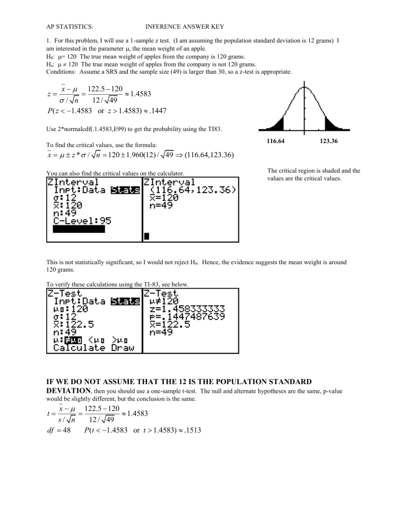
Conditions: Assume a SRS and the sample size (49) is larger than 30, so a z-test is appropriate. z

 x
 
 
1.4583
/ n 12 / 49
 
1.4583 or z

1.4583)

.1447
Use 2*normalcdf(.1.4583,E99) to get the probability using the TI83.
To find the critical values, use the formula: x z *

/ n

120 1.960(12) / 49

(116.64,123.36)
You can also find the critical values on the calculator.
116.64 123.36
The critical region is shaded and the values are the critical values.
This is not statistically significant, so I would not reject H
0
. Hence, the evidence suggests the mean weight is around
120 grams.
To verify these calculations using the TI-83, see below.
, then you should use a one-sample t-test. The null and alternate hypotheses are the same, p-value would be slightly different, but the conclusion is the same. t
 x
  s / n

12 / 49

1.4583
df
  
1.4583 or t

1.4583)

.1513

AP STATISTICS: INFERENCE ANSWER KEY
2. For this problem, I will use a 1-sample t test. I am interested in the parameter

, the mean number of hours per week of part-time work of high school seniors.
H
0
H a
:

= 10.6 The true mean number of hours per week of part-time work of high school seniors is 10.6.
:

10.6 The true mean number of hours per week of part-time work of high school seniors is not 10.6.
Conditions: We are given the data is a SRS and the sample size (50) is larger than 40, so a t-test is appropriate. t
 x
 
 
10.33
s / n 1.3/ 50 df

49 (
 
10.33 or t

10.33)
  
14
Use 2*tcdf(.10.33,E99,49) to get the probability using the TI83.
To find t* = 2.0096, you have to use df = 49 and Table C or the calculator.
10.231 10.969
The critical region is shaded and the values are the critical values.
To find the critical values, use the formula. x * / n

10.6

2.0096(1.3) / 50

(10.231,10.969)
You can also find the critical values on the calculator.
This is statistically significant, so I would reject H
0
. Hence, the evidence suggests the mean number of hours per week of part-time work of high school seniors is not 10.6.
To verify these calculations using the TI-83, see below.

AP STATISTICS: INFERENCE ANSWER KEY
3. For this problem, I will use a 1-sample proportions test. I am interested in the parameter

, the population proportion of defective items.
H
0
H a
:

= 0.03 The true proportion of defective items is 0.03.
:

> 0.03 The true proportion of defective items is greater than 0.03.
Conditions: We are given the data is a SRS, N > 10n, np
0
>10 n(1-p
0
)>10. In checking these conditions, I will assume that the population is ten times as large as the sample size. Second, in checking 250(.03) > 10

7.5> 10 is
NOT satisfied, but 250(.7) > 10

242.5 > 10. Since one of the conditions does not held true, I will proceed with caution. z
 p
0
ˆ  p
0
(1
 p
0
)
 
.1853
n
(

.1853)

.42646
250
Use normalcdf(.1853,E99) to get the probability using the TI83.
This is not statistically significant, so I would not reject H
0
. Hence, the evidence suggests the true proportion of defective items is around 0.03.
To verify these calculations using the TI-83, see below.

AP STATISTICS: INFERENCE ANSWER KEY
4. For this problem, I will use a two-sample t test. I am interested in determining if there is a difference between the mean study times between the two schools are different.
H
0
: u
1
= u
2
The mean study time at the two school are equal.
H a
: u
1
> u
2
The mean study time Driscoll is more than the mean study time at Fenton.
Conditions: We are given the data is a SRS from two different populations. Also, n
1
+ n
2
= 140 > 40. t
 x
1
 x
2
 
.7827
s
1
2
 s
2
2 n
1 n 2
4.35
2

4.87
2
65 75 df

64 (

.7827)

.21834
To get the probability, tcdf(.7827,E99,64) on the TI-83.
This is not statistically significant, so I would not reject H
0
. Hence, the evidence suggests mean study time at both schools is about the same.
To verify these calculations using the TI-83, see below. NOTE: THE CALCULATOR USED THE ADVANCED
DEGREES OF FREEDOM TO CALCULATE THE P-VALUE. THIS IS NOT THE SAME AS ABOVE.

AP STATISTICS: INFERENCE ANSWER KEY
5. For this problem, I will use a matched pairs t-test. I am interested in determining if the SAT test preparation course will improve a students Math SAT score at Fenton by 50 points.
H
0
H a
:

= 50 The SAT test preparation course increased a students Math SAT score by fifty points.
:

> 50 The SAT test preparation course increased a students Math SAT score by more than fifty points.
Conditions: We are given the data is a SRS. The sample size (10) is less than 15,but the normal quantile plot show the data is not non-normal. However, there is an outlier, so I will proceed with caution and be skeptical about my results.
Normal Prob. Plot Box and Whiskers
I calculated the difference between scores (After - Before) to be 25,28,20,65,10,43,8135, -12,38. The mean of this set of data is 33.3 with a standard deviation of 26.39. t
 x
  s / n

26.39 / 10
 
2.001
df
  
1.977)

.9618
To get the probability, tcdf(-1.977,E99,9) on the TI-83.
This is not statistically significant, so I would reject H
0
. Hence, the evidence suggests SAT test preparation course does not improve a Fenton high school students score by more than fifty points.
To verify these calculations using the TI-83, Enter the data into L1 and L2, calculate L3=L2 - L1, and run the test below.

AP STATISTICS: INFERENCE ANSWER KEY
6. For this problem, I will use a 2-sample proportions test. I am interested in determining if the population proportions are the same.
H
0
:

1
H a
:

1
=


2
2
The two proportions of students who intend to pursue post-secondary education are equal.
The two proportions of students who intend to pursue post-secondary education are not equal.
Conditions: We are given the data consist of two SRS. I will assume that each population is ten times as large as the sample size (N > 10n
1
and N > 10n
2
). I also need to check the conditions below (see p. 684) with the pooled phat.
 p
1
 p
2 n
1
 n
2

36


31

67
110

.60909
ˆ 5
60(.60909)

36.54

5 n
1
(1
 p )
 
60(.3909)

23.45

5 n p
2
 
50(.60909)

30.45

5 n
2
(1
 p )
 
50(.3909)

19.54

5
All of the conditions are met. z
 p
1
 p
2
ˆ
(1
 n
1
ˆ
)

ˆ
(1
 n
2
ˆ
)

.609(.3909)
60
 
.21405 or z

.21405)

.8305

.609(.3909)
50
 
.21405
Use 2*normalcdf(.21405,E99) to get the probability using the TI83.
This is not statistically significant, so I would not reject H
0
. Hence, the evidence suggests the true proportion of students that plan to pursue post-secondary education are the same in the urban and suburban high schools.
To verify these calculations using the TI-83, see below.

AP STATISTICS: INFERENCE ANSWER KEY
7. For this problem, I will use a 1-sample z test. I am interested in the parameter

, the mean number of days their room deodorizers last.
H
0
H a
:

= 17.3 The mean number of days their room deodorizers last is 17.3.
:

17.3 The mean number of days their room deodorizers last is not 17.3.
Conditions: Assume a SRS and the sample size (20) is not larger than 40, so a t-test should be used with if there are not any outlier or strong skewness in the data (see p. 606). z

 x
/
  n

2.1/ 20
 
4.472
 
4.472 or z

4.472)
  
6
Use 2*normalcdf(-4.472,E99) to get the probability using the TI83.
To find the critical values, use the formula: x z *

/ n

17.3 1.960(2.1) / 20

(16.37,18.22)
16.38 18.22
You can also find the critical values on the calculator.
The critical region is shaded and the values are the critical values.
This is statistically significant, so I would reject H
0
. Hence, the evidence suggests the average number of days a room deodorizer lasts is not 17.3 days as the company claims.
To verify these calculations using the TI-83, see below.
, then you should use a one-sample t-test. The null and alternate hypotheses are the same, p-value would be slightly different, but the conclusion is the same. t
 x
  s / n

2.1/ 20
 
4.472

4 df

19 (
 
4.472 or t

4.472)
 

AP STATISTICS: INFERENCE ANSWER KEY
8. For this problem, I will use a two-sample t test. I am interested in determining if the Fowler motor lasts longer than the Malloy motor.
H
0
: u
1
= u
2
The Fowler and Malloy motors mean life are equal.
H a
: u
1
> u
2
The mean life of a Fowler motor is larger than the mean life of a Malloy motor.
Conditions: We are given the data is a SRS from two different populations. Also, n
1
+ n
2
= 95 > 40. t
 x
1
 x
2
 s
1
2
 s
2
2 n
1 n 2
2.1
2

2.1
45 50
2
 
1.1587
df

44 (
 
1.1587)

..87359
To get the probability, tcdf(.-1.1587,E99,44) on the TI-83.
This is not statistically significant, so I would not reject H
0
. Hence, the evidence suggests the mean life of the motors are the same.
To verify these calculations using the TI-83, see below. NOTE: THE CALCULATOR USED THE ADVANCED
DEGREES OF FREEDOM TO CALCULATE THE P-VALUE. THIS IS NOT THE SAME AS ABOVE.
12
13
10
11
Problem
9
Parameter of Interest
Mu
P
Mu
P
Mu
Choice of Test
Two-sample t-test
One-sample proportions test
Two sample t-test
Two-sample proportions test
Matched pairs
Null Hypothesis in words
The new halogen bulb lasts twenty five more hours than the incandescent bulb
The population proportion of students who prefer the
Mehta bookbag is .55
The average score on the state test is the same for urban districts and suburban districts
The proportion of males and females going to postsecondary education after graduation are equal.
The difference between the pre-test and post-test scores of third graders is zero.

AP STATISTICS: INFERENCE ANSWER KEY
14. For this problem, I will use a Chi-square, goodness of fit test. I am interested in determining if the proportion of prizes claimed by the manufacturer is the same as the observed proportions.
H
0
: The proportions of getting various prizes claimed by the manufacturer are the same as the observed proportions.
H a
: At least on of the proportions of getting various prizes claimed by the manufacturer are different than the observed proportions.
Conditions: I can use this test if all expected at least 80% of the expected counts are larger than five and all are at least one. The expected counts are in L2, thus the condition is satisfied.
 
 observed
 exp ected exp ected

2

2 
204

306
...
9.693
df
 
2 
9.693)

.0459
To get the probability, use X 2 cdf(9.693,E99,4)
This is statistically not significant at the 5% level. Thus, there is no reason not to believe that the observed proportions are equal to the population proportions.

AP STATISTICS: INFERENCE ANSWER KEY
15. For this problem, I will use a 2-sample proportions test. I am interested in determining the proportion of families that watch the TV show in rural Indiana is the same as the proportion of families that watch the TV show in urban Indiana.
H
0
:

1
H a
:

1
=

2
The two proportions of urban and rural families that watch the TV show are equal.
>

2
The proportion of urban families that watch the TV show is greater than the proportion of rural families that watch the show.
Conditions: We are given the data consist of two SRS. I will assume that each population is ten times as large as the sample size (N > 10n
1
and N > 10n
2
). I also need to check the conditions below (see p. 684) with the pooled phat.
 p
1
 p
2 n
1
 n
2

40


22

62
100 50 150

.41333
n p
1
 
100(.41333)

41.3333

5 n
1
(1
 p )
 
100(.5866)

58.666

5
ˆ 5
50(.41333)

20.666

5 n
2
(1
 p )
 
50(.5866)

29.3333

5
All of the conditions are met. z
 p
1
 p
2
ˆ
(1
 n
1
ˆ
)

ˆ
(1
 n
2
ˆ
)
(

.46897)

.31954

.41333(.58666)
50

.41333(.58666)
100

.46897
Use normalcdf(.46897,E99) to get the probability using the TI83.
This is not statistically significant, so I would not reject H
0
. Hence, the evidence suggests the two proportions f urban and rural families that watch the TV show are equal.
To verify these calculations using the TI-83, see below.