STAT 211
Handout 5 (Chapter 5)
Joint Probability Distributions and Random Samples
By using the following examples, the joint probability mass function for two discrete
random variables and their properties, their marginal probability mass functions, the case
for independent and dependent variables, their conditional distributions, expected value,
variance, covariance, and correlation will be demonstrated. Properties will be explained.
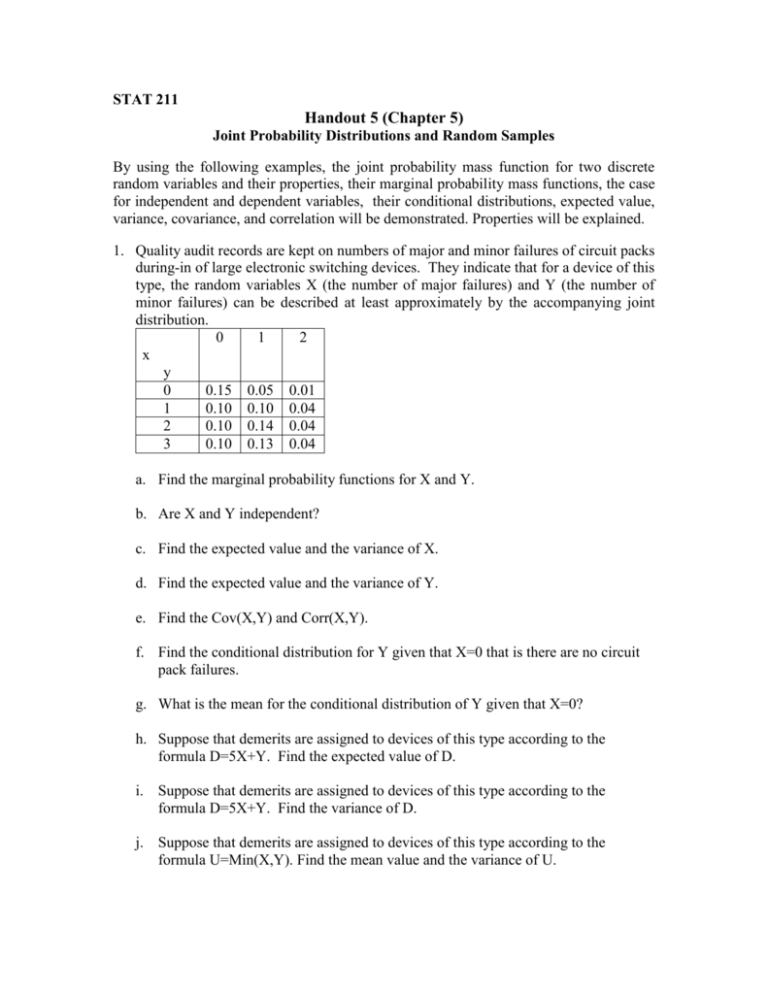
1. Quality audit records are kept on numbers of major and minor failures of circuit packs
during-in of large electronic switching devices. They indicate that for a device of this
type, the random variables X (the number of major failures) and Y (the number of
minor failures) can be described at least approximately by the accompanying joint
distribution.
0
1
2
x
y
0
0.15 0.05 0.01
1
0.10 0.10 0.04
2
0.10 0.14 0.04
3
0.10 0.13 0.04
a. Find the marginal probability functions for X and Y.
b. Are X and Y independent?
c. Find the expected value and the variance of X.
d. Find the expected value and the variance of Y.
e. Find the Cov(X,Y) and Corr(X,Y).
f. Find the conditional distribution for Y given that X=0 that is there are no circuit
pack failures.
g. What is the mean for the conditional distribution of Y given that X=0?
h. Suppose that demerits are assigned to devices of this type according to the
formula D=5X+Y. Find the expected value of D.
i. Suppose that demerits are assigned to devices of this type according to the
formula D=5X+Y. Find the variance of D.
j. Suppose that demerits are assigned to devices of this type according to the
formula U=Min(X,Y). Find the mean value and the variance of U.
By using the following example, the joint probability density function for two continuous
random variables and their properties, their marginal probability density functions, the
case for independent and dependent variables, their conditional distributions, expected
value, variance, covariance, and correlation will be demonstrated. Properties will be
explained.
2. Suppose that a pair of random variables, X and Y have the same joint probability
density
 x(1  y ) if 0  x  2 and 0  y  1
f ( x, y )  
 0 otherwise
a. Find the marginal probability density functions for X and Y.
b. Are X and Y independent?
c. Evaluate P(X+2Y1).
d. Find the expected value and variance of X.
e. Find the expected value and variance of Y.
f. Find the conditional probability function of x given y=0.6.
g. Find the conditional probability function of y given x=0.4.
h. What is E(X|Y=0.6)?
i. Find the Cox(X,Y) and Corr(X,Y).
Random Sample:
The random variables X1, X2, ….,Xn are said to form a random sample of size n if
(i) The Xi's are independent random variables.
(ii) Every Xi's has the same probability distribution.
_
The sampling distribution of x : Discussion theoretically
Exercise 5.42 (textbook): A company maintains 3 offices in a certain region, each
staffed by two employees. Information concerning yearly salaries (1000’s of dollars) is
as follows:
Office
1
1
2
2
3
3
Employee
1
2
3
4
5
6
Salary
19.7 23.6 20.2 23.6 15.8 19.7
(a) Suppose two of these employees are randomly selected from among the six (without
_
replacement). Determine the sampling distribution of the sample mean salary X .
S={(1,2),(1,3),(1,4),(1,5),(1,6),(2,1),(2,3),(2,4),(2,5),(2,6),(3,1),(3,2),(3,4),(3,5),(3,6),
(4,1),(4,2),(4,3),(4,5),(4,6),(5,1),(5,2),(5,3),(5,4),(5,6),(6,1),(6,2),(6,3),(6,4),(6,5)}. There
are 30 outcomes.
_
x
21.65
19.95
17.75
19.70
21.90
23.60
18.0
when
when
when
when
when
when
when
(1,2),(2,1),(1,4),(4,1),(2,6),(6,2),(4,6),(6,4) with 8 outcomes
(1,3),(3,1),(3,6),(6,3) with 4 outcomes
(1,5),(5,1),(5,6),(6,5) with 4 outcomes
(1,6),(6,1),(4,5),(5,4),(2,5),(5,2) with 6 outcomes
(2,3),(3,2),(3,4),(4,3) with 4 outcomes
(2,4),(4,2) with 2 outcomes
(3,5),(5,3) with 2 outcomes
_
x
: 17.75 18
19.7
19.95 21.65 21.90 23.60 otherwise
6/30
4/30
_
P ( x ) : 4/30
_
_
2/30
8/30
4/30
2/30
0
_
E( x )=  x p( x) =613/30=20.43
(b) Suppose one of the three offices is randomly selected. Determine the sampling
_
distribution of the sample mean salary X .
S={(1,2),(2,1),(3,4),(4,3),(5,6),(6,5)}. There are 6 outcomes
_
x
21.65 when (1,2),(2,1) with probability 1/3
21.90 when (3,4),(4,3) with probability 1/3
17.75 when (5,6),(6,5) with probability 1/3
_
E( x )=61.3/3=20.43
Population mean = (19.7+23.6+20.2+23.6+15.8+19.7)/6=20.43
Additional: The sampling distribution of the range of salaries for part (b) in the previous
question is
range:
3.4
3.9
p(range) :
2/6
4/6
E(range)=  range  p(range) =3.7333 where Population range is 23.6-15.8=7.8
The distribution of a linear combination of variables: Discussion theoretically
Exercise 5.60:
First two cars are economy brand and distributed N(20,4)
Last three cars are name brand and distributed N(21,3.5)
All five are independent.
Y is a measure of the difference in efficiency between economy gas and name brand gas.
 X  X 2 X 3  X 4  X 5  20  20 21  21  21


E(Y)= E  1
=20-21=-1
=
2
3
2
3


 X  X 2 X 3  X 4  X 5  4  4 3.5  3.5  3.5

Var(Y)= Var 1
=2+1.6667=3.6667

=
4
9
2
3


P(Y0)=P(Z0.52)=0.3015
P(-1Y1)=P(Y1)-P(Y<-1)=P(Z1.05)-P(Z<0)=0.8531-0.5=0.3531
Exercise 5.66 : (a) 50, 10.308 (b) 0.0075 (c) 50 (d) 111.5625 (e) 50, 131.25
Exercise 5.68: Suppose the speed for the 1st airplane is X1 and the speed for the 2nd
airplane is X2. (a) P(X1-X2 <5)=0.9616 (b) P(0X2-X110)=0.0623
Exercise 5-69: (a) 2400 (b) with independence,1205 (c) 2400, 41.77
Central Limit Theorem: Let X1, X2,….,Xn be a random sample from a distribution with
_
mean  and variance 2. Then if n is sufficiently large (n>30), X has approximately a
normal distribution with mean
   and variance  2   2 / n and
_
_
X
X
approximately a normal distribution with mean 
 xi
The larger the value of n, the better the approximation.
n
X
i 1
i
has
 n and variance  2 x  n 2 .
i
Example: Let X1,X2,…,X100 denote the actual net weights of randomly selected 50-lb
bags of fertilizer. If the expected weight of each bag is 50 and the variance is 1,
(a) What is the probability that the average weight of 100 bags will be between 49.75 and
50.25?
(b) What is the probability that the total weight of 100 bags will be between 4975 and
5025?