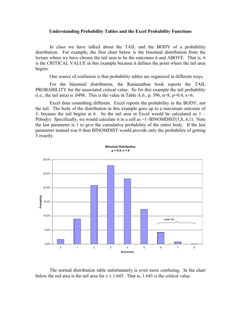
Understanding Probability Tables and the Excel Probability Functions
In class we have talked about the TAIL and the BODY of a probability
distribution. For example, the first chart below is the binomial distribution from the
lecture where we have chosen the tail area to be the outcomes 6 and ABOVE. That is, 6
is the CRITICAL VALUE in this example because it defines the point where the tail area
begins.
One source of confusion is that probability tables are organized in different ways.
For the binomial distribution, the Ramanathan book reports the TAIL
PROBABILITY for the associated critical value. So for this example the tail probability
(i.e., the tail area) is .0498. This is the value in Table A.6., p. 596, n=8, p=0.4, x=6.
Excel does something different. Excel reports the probability in the BODY, not
the tail. The body of the distribution in this example goes up to a maximum outcome of
5, because the tail begins at 6. So the tail area in Excel would be calculated as 1 –
P(body). Specifically, we would calculate it in a cell as =1–BINOMDIST(5,8,.4,1). Note
the last parameter is 1 to give the cumulative probability of the entire body. If the last
parameter instead was 0 then BINOMDIST would provide only the probability of getting
5 exactly.
Binomial Distribution
p = 0.4, n = 8
30.0%
25.0%
Probability
20.0%
15.0%
10.0%
upper tail
5.0%
0.0%
0
1
2
3
4
5
6
7
8
Successes
The normal distribution table unfortunately is even more confusing. In the chart
below the red area is the tail area for z  1.645. That is, 1.645 is the critical value.
Ramanathan in Table A.1 does NOT report the tail probability. He doesn’t report
the entire body probability either. He gives the probability from 0 to the critical value.
Because the standard normal curve is centered at 0, we know that the probability from 0
to infinity is 0.5. The tail probability therefore equals 0.5 minus the value in the table.
Since Table A.1 gives a table value of 0.45 (the midpoint between 1.64 and 1.645), the
tail probability is 0.05.
Ramanathan presents a different normal table in the inside cover of the book (the
table called the percentage points of the t-distribution). Remember I said in class that a tdistribution with infinity degrees of freedom is the same as a normal distribution. If you
look on the last row of this table you will also find 1.645. The very top row gives the
probability in the upper tail, i.e., 0.05.
Excel is a more consistent because it gives the body probability. So a cell with
=NORMSDIST(1.645) gives the value 0.95, which is the total cumulative probability up
to this critical value. The tail probability is then 1 minus this value. In one step, the tail
probability would be =1–NORMSDIST(1.645). [NORMSDIST assumes a standard
normal, with mean 0 and std. deviation 1).]
0.450
0.400
0.350
0.300
f(z)
0.250
0.200
0.150
tail area
0.100
0.050
2.95
2.78
2.61
2.44
2.1
2.27
1.93
1.76
1.59
1.42
1.25
1.08
0.91
0.74
0.4
0.57
0.23
-0.1
0.06
-0.3
-0.5
-0.6
-1
-0.8
-1.1
-1.3
-1.5
-1.6
-2
-1.8
-2.2
-2.3
-2.5
-2.7
-3
-2.8
0.000
z
The moral is you have to be careful when you read tables or use software (different
programs may report tail probs instead of cumulative probs, etc.) The key thing is to
have a good mental picture of the difference between the tail and the body. As we saw in
the gladiolus bulb problem, it is easy to get confused. Unfortunately, this is the way the
world is. But you now have the tools to figure it out!