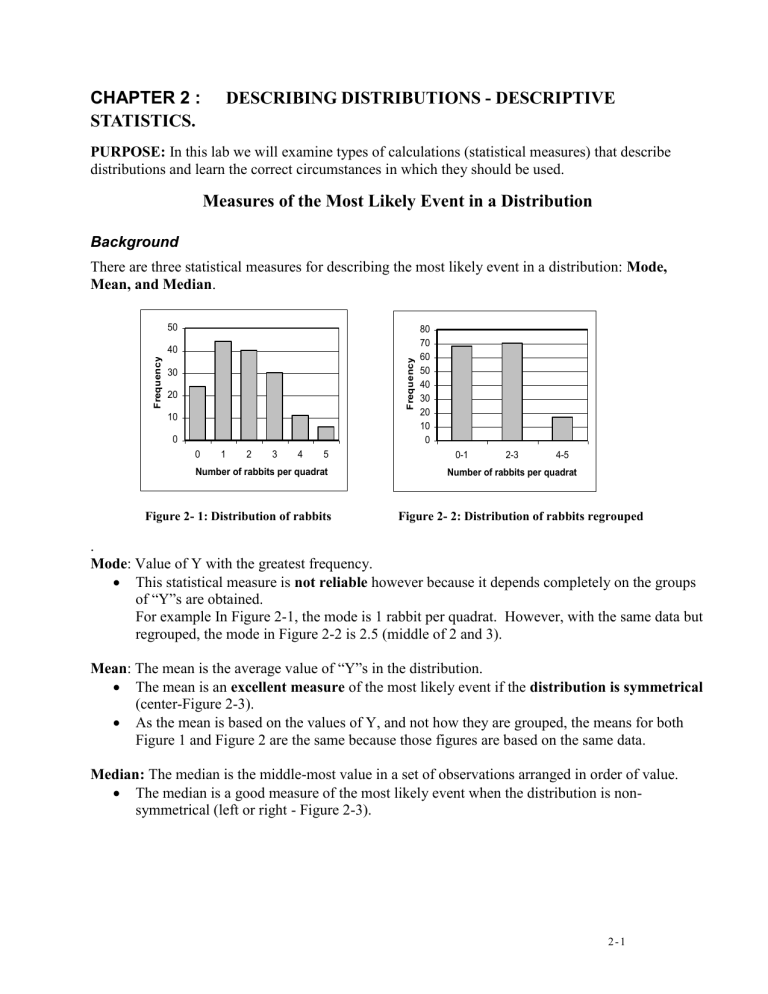
CHAPTER 2 :
STATISTICS.
DESCRIBING DISTRIBUTIONS - DESCRIPTIVE
PURPOSE: In this lab we will examine types of calculations (statistical measures) that describe
distributions and learn the correct circumstances in which they should be used.
Measures of the Most Likely Event in a Distribution
Background
There are three statistical measures for describing the most likely event in a distribution: Mode,
Mean, and Median.
50
Frequency
Frequency
40
30
20
10
0
0
1
2
3
4
5
Number of rabbits per quadrat
Figure 2- 1: Distribution of rabbits
80
70
60
50
40
30
20
10
0
0-1
2-3
4-5
Number of rabbits per quadrat
Figure 2- 2: Distribution of rabbits regrouped
.
Mode: Value of Y with the greatest frequency.
 This statistical measure is not reliable however because it depends completely on the groups
of “Y”s are obtained.
For example In Figure 2-1, the mode is 1 rabbit per quadrat. However, with the same data but
regrouped, the mode in Figure 2-2 is 2.5 (middle of 2 and 3).
Mean: The mean is the average value of “Y”s in the distribution.
 The mean is an excellent measure of the most likely event if the distribution is symmetrical
(center-Figure 2-3).
 As the mean is based on the values of Y, and not how they are grouped, the means for both
Figure 1 and Figure 2 are the same because those figures are based on the same data.
Median: The median is the middle-most value in a set of observations arranged in order of value.
 The median is a good measure of the most likely event when the distribution is nonsymmetrical (left or right - Figure 2-3).
2-1
Skewed right
Skewed left
Non-symmetrical
Symmetrical
Non-symmetrical
Figure 2- 1: Skewness
Computing Measures of the Most Likely Event
We will NOT include computations for the mode because there are none. You just identify the group
with the highest frequency,
There are two types of equations for each measure:
1) Parametric measure. This is the real value or parameter of the population.
2) Sample measure. This is an estimate of the real value based on a sample.
In addition, there are computations for raw data and data grouped into frequencies. If you have a
large number of observations (>50), it is easier to use the computation for data grouped into
frequencies. The appropriate choice depends on how much work you want to do to get the answer.
2-2
Mean: The mean is the average of “Y”s.
Parametric Mean – When you have measurements for the ENTIRE population. The symbol for the parametric mean = μ.
Raw Data (not in frequencies)
Formula:  
Y
where N is
N
the number of individuals in the
population.
Y  1+10+4+
Example
Data:
7+2+6 = 30
Y= 1, 10, 4, 7,
2, 6
N=6
observations

Y
N
 5.0
Frequency Data with single value classes
Formula:  
  f * Y  where f

f
Example Data:
Example Computations
Frequency
(f)
24
44
40
30
11
6
 f 155
Y
0
1
2
3
4
5
TOTAL
=N
f*Y
There were 24+44+40+30+11+6=155 observations =N
  f . The frequencies indicate that these 155 values
are composed of twenty-four “0”s, forty-four “1”s, forty
“2”s, thirty “3”s, eleven “4”s and six “5”s.
24*0 = 0
44*1 = 44
40*2 = 80
The sum would then be
30*3 = 90
11*4 = 44
(24*0) + (44*1) + (40*2) + (30*3) + (11*4) + (6*5)
6*5 = 30
   f * Y   288.


f
*
Y

288

  f * Y   288  1.86

155
f
Frequency Data with range of value classes
Example Data:
Class
0.0 – 0.9
1.0 - 1.9
2.0 – 2.9
3.0 – 3.9
4.0 – 4.9
TOTAL
Example Computations
Class
Mark
(Y)
0.45
1.45
2.45
3.45
4.45
Frequency
(f)
2
10
13
7
1
 f 33
f*Y
0.9
14.5
31.85
24.15
4.45
 f  33 which means there were 33 observations (N=33).
  f * Y  75.85 which means that the total of all observations = 72.85
  f * Y   72.85  2.298

33
f
  f * Y  75.85
2-3
Sample Mean – An estimate of the parametric mean from a sample. The symbol for the sample mean = Y .
Raw Data (not in frequencies)
Formula: Y 
 Y where n is the number of individuals in
n
Frequency Data
Formula: Y 
the sample.
  f * Y  where f

f
=n
Example Data and Computation
Example Data and Computation
The computation is identical to the computation for the
parametric mean.
The computation is identical to the computation for the parametric mean.
Median: The middlemost value in a set of ordered observations.
Parametric and Sample Median – The computations are the same if you are measuring the entire population or estimating the
median from a sample.
Odd Number of Observations
Even Number of Observations
Formula: M  Y0.5*( N 1) where N is the number of observations
Formula: M  Y0.5*( N 1) where N is the number of observations
Example Data: Y= 15, 4, 2, 8, 11
Example Data: 22,1,12,6,8,5.
Example Computation:
Example Computation:
1) Put observations in order:
1) Put observations in order:
2, 4, 8, 11, 15
2) M  Y0.5*(51)  Y3
1, 5, 6, 8, 12, 22
which means that M is the third
observation.
2, 4, 8, 11, 15
2-4
So M=8
2) M  Y0.5*( 61)  Y3.5  which means that the median is halfway in
between the values for observations Y3 and Y4
3) Y3 =6 and Y4 = 8 so M is halfway in between or M 
68
7
2
Parametric and Sample Median of Frequency Data - The number of the observation to use for M is determined using the same formula
as for raw data. The difference is in locating the value because the data in a frequency table are already in order.
Frequency Data with single value classes
Example Data:
Example Computations:
Y
Frequency
Observations
0
5
Y1 to Y5
1
10
Y6 to Y15
2
3
Y16 to Y18
3
1
Y19
TOTAL
f
1)
f
 N  19 so M  Y0.5*(191)  Y10
2) The 10th observation is found in the class (Y) where Y=1 so M=1
19
Frequency Data with range of value classes
Example Data:
Example Computations:
f
 N  33 so M  Y0.5*(331)  Y17
0.0 – 0.9
Class Mark
(Y)
0.45
1.0 - 1.9
1.45
10
th
Y1 to Y2 2) The 17 observation is found in the class with class mark 2.45 so
M=2.45
Y3 to Y12
2.0 – 2.9
2.45
13
Y13 to Y25
3.0 – 3.9
3.45
7
Y26 to Y32
4.0 – 4.9
TOTAL
4.45
1
Y33
Class
Frequency (f)
2
f
Observations
1)
33
2-5
Measures of Variation in a Distribution.
There are three statistical measures for describing the variation in a distribution: Range, Variance
(and standard deviation), and the Interquartile Distance.
The range is typically associated with a mode, the variance is associated with a mean and the
interquartile distance is associated with a median.
Range: The range is simply the difference between the largest value and the smallest value in a data
set.

The range is a very poor measure of variation because it only includes two observations
Variance: The variance is measured in conjunction with the mean. It is a measure based on the
differences between the mean and each value.
 This statistical measure is an excellent measure of variation when the distribution is
symmetrical.
 The standard deviation is the square root of the variance and is also used as a measure of
variation that is in the same units as the mean (i.e. not squared).
Interquartile Distance: This measure is used in conjunction with the median. It is the range between
the first fourth of the data and the last fourth of the data.
 The interquartile distance is a good measure of variation for non-symmetrical distributions.
Computing Measures of Variation
There are two types of equations for each measure, one for the real value on an entire population
(Parametric statistical measure) and one for an estimate of the real value based on a sample (Sample
statistical measure).
In addition, there are computations for raw data and data grouped into frequencies.
2-6
Range: Difference between the highest and lowest value.
Range for parametric and sample data - The computations are the same if you are measuring the entire population or estimating
the range from a sample.
Formula: Highest value – lowest value
Raw data: Y= 1, 10, 4, 7, 2, 6
Range = 10-1=9
Variance: Average squared difference between each value and the mean.
Variance for parametric data – The symbol for parametric variance =  2
Raw Data (not in frequencies)
 Y   

Frequency Data with single value classes
2
Formula: 
2
which is
N
also equal to
Y 2 
Formula:  
( Y ) 2
N
where N is the
N
number of individuals in the population.
2 
Example
Data:
Y= 1, 10,
4, 7, 2, 6
  f *Y
2
Example Computations:
Y
 1 + 10 + 4 + 7 +
22 + 62 = 206
2
2
2
2
2
Y  30
N=6
2 
2
30
6  56  9.333
6
6
206 
    f * Y 
2
2
f
f
f
where
Example Data:
Y
0
1
2
3
4
5
Frequency (f)
24
44
40
30
11
6
 f 155
=N
Example Computations:
f*Y
f*Y2
24*0 = 0
24*02=0
44*1 = 44
44*12=44
40*2 = 80
40*22=160
30*3 = 90
30*32=270
11*4 = 44
11*42=176
6*5 = 30
6*52=150
  f * Y    f *Y 2 
=288
=800


 f  155 (N=155).
  f * Y   288   f * Y  800
2
2 
288 2
155  264.877  1.709
155
155
800 
2-7
Variance for sample data –An estimate of the parametric variance from a sample. The symbol for the sample variance =s2.
Raw Data (not in frequencies)
 Y  Y 

Frequency Data with single value classes
2
Formula: 
2
also equal to
Y 2 
Formula: s 
2
( Y ) 2
n
where n is the
n 1
number of individuals in the sample.
2 
  f *Y
which is
n 1
NOTE that
    f * Y 
2
2
 f 1
f
where
f
=n
 f 1 is in the denominator which is an adjustment to correct for
underestimating the variance
NOTE that n-1 is in the denominator
which is an adjustment to correct for
underestimating the variance
Example
Data:
Y= 1, 10,
4, 7, 2, 6
Example Computations:
Y
 1 + 10 + 4 + 7 +
2 + 6 = 206
2
2
2
2
2
2
2
Y  30
n=6
2 
30 2
6  56  11.2
5
5
206 
Example Data:
Y
0
1
2
3
4
5
Frequency (f)
24
44
40
30
11
6
 f 155
Example Computations:
f*Y
f*Y2
24*0 = 0
24*02=0
44*1 = 44
44*12=44
40*2 = 80
40*22=160
30*3 = 90
30*32=270
11*4 = 44
11*42=176
6*5 = 30
6*52=150
  f * Y    f *Y 2 
=288
=800


 f  155 (n =155).
  f * Y   288   f * Y  800
2
288 2
800 
155  264.877  1.720
s2 
154
154
NOTE that the difference between the parametric and sample variance is large when sample size is small but the difference is
smaller with a larger n. In our examples with n=6,  2 =9.333 but s2=11.2. However, with n=155,  2 =1.709 and s2=1.72
That is because, the larger the sample size, the less likely it is that you will underestimate the parametric variance.
2-8
Standard Deviation: Square root of the variance.
Standard deviation for parametric data - The computation is also the same if you are using raw or frequency data.
Parametric Data – The symbol for Standard Deviation = 
Estimate from Sample Data – The symbol for sample Standard
Deviation = s
Formula:    2
Formula: s  s 2
Example Data:
Example Computations:
Example Data:
Example Computations:
 2  9.333
  9.333  3.055
s 2  11.2
s  11.2  3.347
Interquartile distance: The difference between the third and first quartile.
Parametric and Sample Interquartile Distance – The computations are the same if you are measuring the entire population or
estimating the median from a sample.
Formula: IQD  Y0.75*( N 1)  Y0.25*( N 1) where N is the number of observations.
Raw Data
Example Data: Y= 15, 4, 2, 8, 11
Example Computations:
1) Put observations in order:
2, 4, 8, 11, 15
2) 3rd quartile  Y0.75*(51)  Y4.5
which means that the third
quartile is halfway between the 4th and 5th observations.
3) Y4 =11 and Y5 = 15 so the 3rd quartile is halfway in between
11  15
 13
or Q3 
2
4) 1st quartile  Y0.25*(51)  Y1.5
which means that the third
quartile is halfway between the 1st and 2nd observations.
5) Y1 =2 and Y2 = 4 so the 1st quartile is halfway in between or
24
Q1 
3
2
6) The IQD = Q3-Q1 = 13-3 = 10
2-9
Parametric and Sample Interquartile Distance of Frequency Data
Frequency Data with single value classes
The number of the observation to use for M is determined using the same formula as for raw data. The difference is in locating the value
because the data in a frequency table are already in order
Example Data:
Example Computations:
Y
Frequency
Observations
0
6
Y1 to Y6
1
12
Y7 to Y18
2
2
Y19 to Y20
3
2
Y21 to Y22
4
1
Y23
12
1
Y24
TOTAL
f
24
1)
f
 N  24 so Q3  Y0.75*(241)  Y18.75
which means that
the third quartile is three quarters of the way between the 18th
and 19th observations.
2) Y18 =1 and Y19 = 2. Three quarters of the way =
Y18  (Y19  Y18 ) * 0.75  1  1* 0.75  1.75 so the 3rd quartile is
Q3  1.75
3) Q1  Y0.25*(241)  Y6.25
which means that the third quartile is
one quarter of the way between the 6th and 7th observations.
4) Y6 =0 and Y7 = 1. One quarter of the way =
Y6  (Y7  Y6 ) * 0.25  0  1* 0.25  0.25 so the 1st quartile is
Q3  0.25
5) The IQD = Q3-Q1 = 1.75-0.25 = 1.5
Frequency Data with range of value classes – The computation is virtually the same as for single value classes but you use the class
marks as Y
2-10
On your own - Most Likely Event in a Distribution
1) Why is it so important to use the correct symbols for sample statistics ( Y , s2) and parametric
statistics (e.g. , 2).
2) Compute the sample mean of the following: 1.2, 3.1, 1.0, 6.4, 2.1
3) Compute the median of the data in question 2.
4) Compute the sample mean and variance for the following:
Class
0.1 – 0.5
0.6 – 1.0
1.1 – 1.5
1.6 – 2.0
2.1 – 2.5
Class
Mark
(Y)
Frequency
(f)
f*Y
f*Y2
Observations
8
10
8
22
2
5) Compute the median of the data in Question 4:
6) Compute the median of the following: 1.2, 3.1, 1.0, 6.4, 2.1, 7.8
2-11
7) Compute the interquartile distance for the data in question 6.
8) Given the information in the following figure, would you compute the mean or the median?
9) You would like determine how variable tree height is in a forest that had been burned several
years previously. You randomly selected 300 trees and, to make your job easier, you placed
trees in one of 10 height classes rather than taking a precise measurement for each tree. You
counted the number of trees in each height class and determined that the distribution of
heights was symmetrical. What is the appropriate measure and what is the appropriate
equation?
10) You are using a nephalometer to measure water clarity in a lake. You have taken several
measurements and want to know the most likely value for water clarity. In your
measurements there were a few very high readings. What is the appropriate measure and
what is the appropriate equation?
11) What is the difference between “N” in the equation for the parametric mean and “n” in the
equation for the sample mean?
2-12
2-13