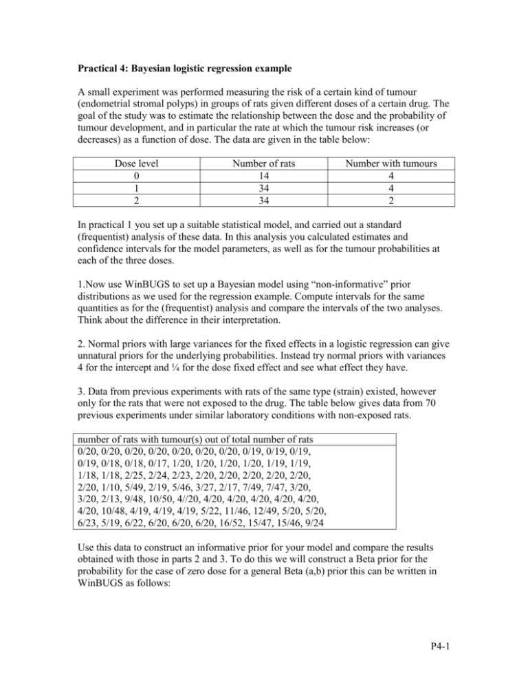
Practical 4: Bayesian logistic regression example
A small experiment was performed measuring the risk of a certain kind of tumour
(endometrial stromal polyps) in groups of rats given different doses of a certain drug. The
goal of the study was to estimate the relationship between the dose and the probability of
tumour development, and in particular the rate at which the tumour risk increases (or
decreases) as a function of dose. The data are given in the table below:
Dose level
0
1
2
Number of rats
14
34
34
Number with tumours
4
4
2
In practical 1 you set up a suitable statistical model, and carried out a standard
(frequentist) analysis of these data. In this analysis you calculated estimates and
confidence intervals for the model parameters, as well as for the tumour probabilities at
each of the three doses.
1.Now use WinBUGS to set up a Bayesian model using “non-informative” prior
distributions as we used for the regression example. Compute intervals for the same
quantities as for the (frequentist) analysis and compare the intervals of the two analyses.
Think about the difference in their interpretation.
2. Normal priors with large variances for the fixed effects in a logistic regression can give
unnatural priors for the underlying probabilities. Instead try normal priors with variances
4 for the intercept and ¼ for the dose fixed effect and see what effect they have.
3. Data from previous experiments with rats of the same type (strain) existed, however
only for the rats that were not exposed to the drug. The table below gives data from 70
previous experiments under similar laboratory conditions with non-exposed rats.
number of rats with tumour(s) out of total number of rats
0/20, 0/20, 0/20, 0/20, 0/20, 0/20, 0/20, 0/19, 0/19, 0/19,
0/19, 0/18, 0/18, 0/17, 1/20, 1/20, 1/20, 1/20, 1/19, 1/19,
1/18, 1/18, 2/25, 2/24, 2/23, 2/20, 2/20, 2/20, 2/20, 2/20,
2/20, 1/10, 5/49, 2/19, 5/46, 3/27, 2/17, 7/49, 7/47, 3/20,
3/20, 2/13, 9/48, 10/50, 4//20, 4/20, 4/20, 4/20, 4/20, 4/20,
4/20, 10/48, 4/19, 4/19, 4/19, 5/22, 11/46, 12/49, 5/20, 5/20,
6/23, 5/19, 6/22, 6/20, 6/20, 6/20, 16/52, 15/47, 15/46, 9/24
Use this data to construct an informative prior for your model and compare the results
obtained with those in parts 2 and 3. To do this we will construct a Beta prior for the
probability for the case of zero dose for a general Beta (a,b) prior this can be written in
WinBUGS as follows:
P4-1
p0 ~ dbeta(a,b)
beta0 <- logit(p0)
Consider the following two approaches to construct values for a and b
a) Ignore the fact that the results are from many different experiments and are
therefore subject to clustering and combine the data into a Beta(x+1,n-x+1) prior
where x is the total number of positives and n is the total number of animals. Note
this would only really be sensible if the prior data came from a single experiment.
b) Calculate the proportion positive in each experiment and then calculate the mean
and variance of these proportions.
Given the formulae for the mean and variance of a Beta distribution we can
construct the values of a and b from the sample data by matching means and
variances
This gives us the formulae a=m([m(1-m)/v]-1), b=a(1-m)/m
Note if you do not have time to evaluate the mean and variance then these take
values 0.136 and 0.01071 respectively.
P4-2