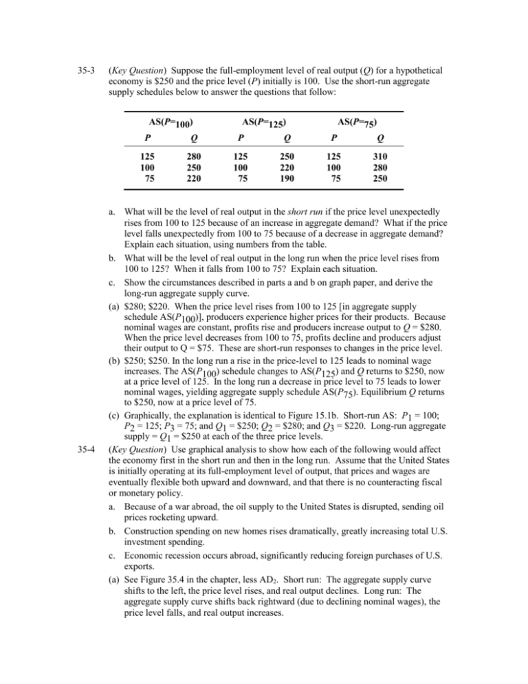
35-3
(Key Question) Suppose the full-employment level of real output (Q) for a hypothetical
economy is $250 and the price level (P) initially is 100. Use the short-run aggregate
supply schedules below to answer the questions that follow:
AS(P=100)
P
Q
125
100
75
35-4
280
250
220
AS(P=125)
P
Q
125
100
75
250
220
190
AS(P=75)
P
Q
125
100
75
310
280
250
a. What will be the level of real output in the short run if the price level unexpectedly
rises from 100 to 125 because of an increase in aggregate demand? What if the price
level falls unexpectedly from 100 to 75 because of a decrease in aggregate demand?
Explain each situation, using numbers from the table.
b. What will be the level of real output in the long run when the price level rises from
100 to 125? When it falls from 100 to 75? Explain each situation.
c. Show the circumstances described in parts a and b on graph paper, and derive the
long-run aggregate supply curve.
(a) $280; $220. When the price level rises from 100 to 125 [in aggregate supply
schedule AS(P100)], producers experience higher prices for their products. Because
nominal wages are constant, profits rise and producers increase output to Q = $280.
When the price level decreases from 100 to 75, profits decline and producers adjust
their output to Q = $75. These are short-run responses to changes in the price level.
(b) $250; $250. In the long run a rise in the price-level to 125 leads to nominal wage
increases. The AS(P100) schedule changes to AS(P125) and Q returns to $250, now
at a price level of 125. In the long run a decrease in price level to 75 leads to lower
nominal wages, yielding aggregate supply schedule AS(P75). Equilibrium Q returns
to $250, now at a price level of 75.
(c) Graphically, the explanation is identical to Figure 15.1b. Short-run AS: P1 = 100;
P2 = 125; P3 = 75; and Q1 = $250; Q2 = $280; and Q3 = $220. Long-run aggregate
supply = Q1 = $250 at each of the three price levels.
(Key Question) Use graphical analysis to show how each of the following would affect
the economy first in the short run and then in the long run. Assume that the United States
is initially operating at its full-employment level of output, that prices and wages are
eventually flexible both upward and downward, and that there is no counteracting fiscal
or monetary policy.
a. Because of a war abroad, the oil supply to the United States is disrupted, sending oil
prices rocketing upward.
b. Construction spending on new homes rises dramatically, greatly increasing total U.S.
investment spending.
c. Economic recession occurs abroad, significantly reducing foreign purchases of U.S.
exports.
(a) See Figure 35.4 in the chapter, less AD2. Short run: The aggregate supply curve
shifts to the left, the price level rises, and real output declines. Long run: The
aggregate supply curve shifts back rightward (due to declining nominal wages), the
price level falls, and real output increases.
35-5
35-7
(b) See Figure 35.3. Short run: The aggregate demand curve shifts to the right, and both
the price level and real output increase. Long run: The aggregate supply curve shifts
to the left (due to higher nominal wages), the price level rises, and real output
declines.
(c) See Figure 35.5. Short run: The aggregate demand curve shifts to the left, both the
price level and real output decline. Long run: The aggregate supply curve shifts to
the right, the price level falls further, and real output increases.
(Key Question) Between 1990 and 2007 the U.S. price level rose by about 61 percent
while real output increased by about 63 percent. Use the aggregate demand-aggregate
supply model to illustrate these outcomes graphically.
In the graph shown, both AD and AS expanded over the 1990-2005 period. Because
aggregate supply increased as well as aggregate demand, the new equilibrium output rose
at a faster pace than did the price level. P2 is 50% above P1 and GDP2 is 56% greater
than GDP1.
(Key Question) Suppose the government misjudges the natural rate of unemployment to
be much lower than it actually is, and thus undertakes expansionary fiscal and monetary
policy to try to achieve the lower rate. Use the concept of the short-run Phillips Curve to
explain why these policies might at first succeed. Use the concept of the long-run
Phillips Curve to explain the long-run outcome of these policies.
In the short-run there is probably a tradeoff between unemployment and inflation. The
government’s expansionary policy should reduce unemployment as aggregate demand
increases. However, the government has misjudged the natural rate and will continue its
expansionary policy beyond the point of the natural level of unemployment. As
aggregate demand continues to rise, prices begin to rise. In the long-run, workers
demand higher wages to compensate for these higher prices. Aggregate supply will
decrease (shift leftward) toward the natural rate of unemployment.
In other words, any reduction of unemployment below the natural rate is only temporary
and involves a short-run rise in inflation. This, in turn, causes long-run costs to rise and a
decrease in aggregate supply. The end result should be an equilibrium at the natural rate
of unemployment and a higher price level than the beginning level. The long-run Phillips
curve is thus a vertical line connecting the price levels possible at the natural rate of
unemployment found on the horizontal axis. (See Figure 35.11)
35-9
(Key Question) What is the Laffer Curve, and how does it relate to supply-side
economics? Why is determining the location where the economy is on the curve so
important in assessing tax policy?
Economist Arthur Laffer observed that tax revenues would obviously be zero when the
tax rate was either at 0% or 100%. In between these two extremes would have to be an
optimal rate where aggregate output and income produced the maximum tax revenues.
This idea is presented as the Laffer Curve shown in Figure 35.12.
The difficult decision involves the analysis to determine what is the optimum tax rate for
producing maximum tax revenue and the related maximum economic output level.
Laffer argued that low tax rates would actually increase revenues because low rates
improved productivity, saving and investment incentives. The expansion in output and
employment and thus, revenue, would more than compensate for the lower rates.