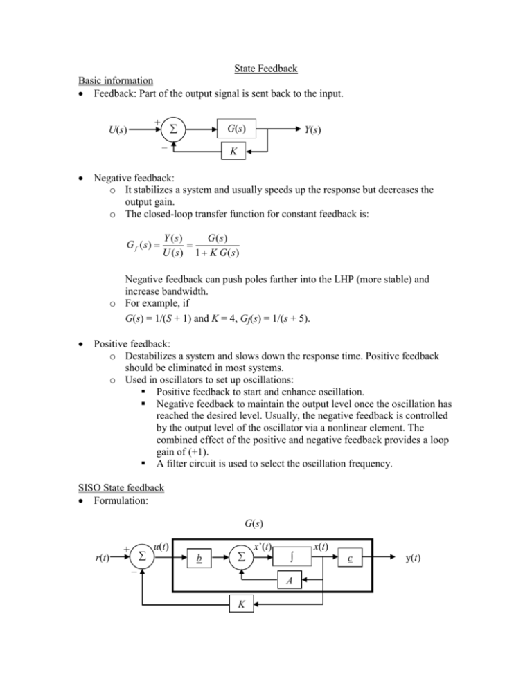
State Feedback
Basic information
 Feedback: Part of the output signal is sent back to the input.
+
U(s)

G(s)
–

Y(s)
K
Negative feedback:
o It stabilizes a system and usually speeds up the response but decreases the
output gain.
o The closed-loop transfer function for constant feedback is:
G f (s) 
Y (s)
G(s)

U (s) 1  K G (s)
Negative feedback can push poles farther into the LHP (more stable) and
increase bandwidth.
o For example, if
G(s) = 1/(S + 1) and K = 4, Gf(s) = 1/(s + 5).

Positive feedback:
o Destabilizes a system and slows down the response time. Positive feedback
should be eliminated in most systems.
o Used in oscillators to set up oscillations:
 Positive feedback to start and enhance oscillation.
 Negative feedback to maintain the output level once the oscillation has
reached the desired level. Usually, the negative feedback is controlled
by the output level of the oscillator via a nonlinear element. The
combined effect of the positive and negative feedback provides a loop
gain of (+1).
 A filter circuit is used to select the oscillation frequency.
SISO State feedback
 Formulation:
G(s)
r(t)
+

u(t)
b

–
x’(t)

A
K
x(t)
c
y(t)
x’ = (A – b K) x + b u = Af x + b u
y =cx
G(s) = c (sI – A)-1 b
Gf(s) = c (sI – A + b K)-1 b = c (sI – Af)-1 b

(A – b K, b) controllable  (A, b) controllable. Although controllability is invariant
under state feedback, observability is not necessarily invariant under state feedback.
State feedback does not affect the zeroes of G(s). It only shifts the position of the
poles.
The eigenvalues can be repositioned by applying state feedback with an appropriate
gain matrix K.
Example:


2
 1
8.1
1
1
 b   
1
2
A  
c  ( 1 1 )
2

 1
1
 2  K1 1  K2 
     ( K1 K2 ) 

1 2
 1  2 K1 1  2 K2 
1
 s 0    2  K1 1  K2   s  2  K1 1  K2 
  
 

 0 s   1  2 K1 1  2 K2   1  2 K1 s  1  2 K2 
 s  2  K1 1  K2 


 1  2 K1 s  1  2 K2 
2
s  3 s  2 s  K2  3  5 K2  K1 s  K1
2
s  ( 3  2 K2  K1)  s  ( 5 K2  3  K1)
lsolve
K1  5 K2 1

2
s  3 s  2
 1 2    6    4 
    
 1 5   1   1 
K1  2 K2 6

( s  1) ( s  2)
The direct evaluation technique, however, becomes rather tedious for higher
dimensional systems.
A more systematic approach is needed. For a controllable system, we can use the
controllability matrix to compute the gain matrix (text, p. 235)
Example:
8.2
 2 1  b   1 

 
 1 1 
2
c  ( 1 1 )
s 0   2 1

 

 0 s   1 1 
s  3 s  3
A  

2
_f
k_  [ 3  ( 3) 2  3 ] k_  ( 6 1 )
1
1 3 

C_  

0 1 
C_  
C  augment ( b  A  b )
C

1
k  k_  C_  C

1 3

0 1
1 4

2 1
k  (4 1)
( s  1) ( s  2)
2
s  3 s  2
P. 236, (8.10) & (8.11)
C_
1
1
C
 1 3 

0 1 

P. 235, (8.9)
 0.143 0.571 

 0.286 0.143 

P. 236, (8.13)
Example:
 1 1 2 
1


A  0 1 1
b   0 


 
0 0 1 
1
 s 0 0   1 1 2 
0 s 0  0 1 1 


 

0 0 s  0 0 1 
k_  [ 4  ( 3) 6  3 4  ( 1) ]
8.4
_f
k_  ( 7 3 5 )
( s  1)
( s  2)  ( s  1  j)  ( s  1  j)
3
3
3
2
s  3 s  3 s  1
2
s  4 s  6 s  4


2
C  augment b  augment A  b  A  b


1
k  k_  C_  C


k  ( 15 47 8 )
1
 1 3 3 
C_   0 1 3 


0
0
1


 1 1 2 
C 0 1 2 


1
1
1


Lyapunov Equation: Every eigenvalue of the feedback system must be different from
that of the original system.
1) Select F (n  n): Use the modal form of Af
2) Select k (1  n): At least one nonzero entry associated with each diagonal block
(text, p. 241)
3) Solve the unique T in the Lyapunov equation: A T – T F = b k
4) k = k T-1
Example: F and k are pre-selected (P. 241)
8.3
 2 1  b   1 

 
 1 1 
2
A  
 1 0 

 0 2 
F  
c  ( 1 1 )
k_  ( 1 1 )
1 1

2 2
b  k_  
 2 1    t11 t12    t11 t12    1 0   3 t11  t21 4 t12  t22   1 1 


 

 
 

 1 1   t21 t22   t21 t22   0 2   t11  2 t21 t12  3 t22   2 2 


 3 1    1   lsolve 4 1    1 T   0 0.077 
  

    

 1 2   2 
 1 3   2    1 0.692 
T  augment  lsolve
k  k_  T
1
k  (4 1)

 placement:
o The controllability condition is the necessary and sufficient condition for the
placement of s to any desired locations.
o Criteria: rise/fall time (response time), settling time, overshoot, …
o Guide: Place all s inside a region:
Im
r


Re

- Large   fast response
- Large r  fast response, large input (low gain), and large BW (more noise)
- Large   large overshoot
- If s are too close together, the response will be slow and the required input will
be large. Hence, s should be placed evenly along an arc.
 Discrete-time systems: The discussion applies directly except for the pole placement
region, which can be obtained from the z = es transformation (Fig. 8.3b, p. 239).
Regulation and tracking
 Regulator problem: If the reference signal is zero [r(t) = 0] and the system is
disturbed by some nonzero initial conditions, we need to find a state feedback gain to
ensure that the response dies out at a desired rate.
 Tracking problem: If the reference signal is a constant [r(t) = a], we need to find a
state feedback gain to ensure that the response approaches r(t) = a as t approaches
infinity. This is also called asymptotic tracking of a step reference input.
 If a = 0 then this becomes the regulator problem.
 If s are inside a sector the disturbed response will die out quickly. No state feedback
is needed. Otherwise, we can use state feedback to shift the s inside a sector.
 The tracking problem: Tracking is possible if the G(s) has no zero at s = 0.
 In addition to state feedback, tracking requires a feedforward path u(t) = pr(t) – k x .
The calculation of the feedforward gain is illustrated below:
8.7 This is the same problem as 8.4
2) ( s
 _f ( s
1
j ) ( s
s 0 0
G( s )
1
c
j ) s
1 1
3
2
(2 0 0 )
4s
2
1
1
(2 0 0 ) 0 s 0
0 1 1
 0
0 0 s
0 0 1
1
2s
G( s )
s
3
8s
2
3s
2
3s
8
1
p
4
8
6s
p  0.5
4