MGMT 201: Statistics
Hypothesis Testing (ASW Chapter 9)

What is hypothesis testing?

We want to examine whether premises about a population are likely to be true (or false).

Specifically, we proceed as follows.
 1. We establish a null hypothesis , which may be as simply as H
0
:
 
10.
 2. We specifically the alternative hypothesis , which is the complement of the null hypothesis. H a
:

The alternative hypothesis is chosen to be our research hypothesis.


> 10.
Suppose, for example, that we are interested in whether a company’s stock is performing better under new managers. Previously, the stock averaged 1.14% per month after adjusting for risk. H
0
:
 
1.14% and H a
:

> 1.14%.

3. We examine a sample to determine the probability that the null hypothesis is true.

Notes:

We will never to be able to conclude something with certainty.

The null is given the benefit of the doubt. That is, we look for somewhat conclusive evidence that the null is incorrect.

Three cases

1. H
0

2. H
 3. H
0
0
:

:

Suppose H
0

:





:

=


 Suppose that
0
0
0
; H a
:

; H a
:

>

<

; H a
:
  

Type I and Type II Errors
10 and H a
:

0
0
0
> 10.

=8.6. If we reject the null hypothesis, we are mistaken. Such an error is called a Type I Error . Specifically, a type I error occurs when we incorrectly reject the null hypothesis.
 Suppose instead that

=12.1. If we fail to reject the null hypothesis, we are mistaken. Such an error is called a Type II Error . Specifically, a type II error occurs when we incorrectly fail




This is the same

we used in previous chapters and is called the level of significance .


 to reject the null hypothesis.
probability of making a type I error.
probability of making a type II error

In many cases, we do not know

. It is difficult to determine because we do not know the population parameters.

Testing Hypotheses

One-Tailed Tests: Large Samples

When 1) H
0
:
  
0
; H a
:

>

0
…or… 2) H
0
:
  
0
; H a
:

<

0
, we must perform a one-tailed test. We reject the null only if the sample mean is significantly away from the hypothesized mean on a pre-specified side. For example, in case I, we reject the null if and only if the sample mean is significantly greater than

0
. In case II, we reject the null if and only if the sample mean is significantly less than

0
.
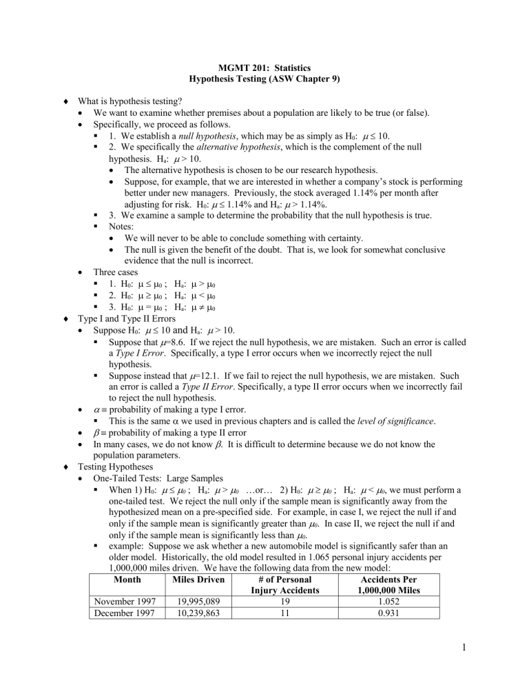
 example: Suppose we ask whether a new automobile model is significantly safer than an older model. Historically, the old model resulted in 1.065 personal injury accidents per
1,000,000 miles driven. We have the following data from the new model:
Month Miles Driven
November 1997
December 1997
19,995,089
10,239,863
# of Personal
Injury Accidents
19
11
Accidents Per
1,000,000 Miles
1.052
0.931
1

January 1998
…
December 2000
14,056,370
…
19,799,440
15
…
18
0.937
…
1.100
January 2001 17,848,493 16 1.116
February 2001
 H
0
:
14,446,470
 
1.065; H a
:

< 1.065
12 1.204

How do we proceed? We simply calculate the z-score of

(1.065 in this case) and the sampling distribution of x . x given the hypothesized
 In this case, n = 40,

Then, z
 x

1 .
065 x = 1.024, s = 0.1379, and s = 0.0218. x

1 .
024

1 .
065
 s x
0 .
0218

1 .
878 . This tells us that the sample mean is 1.878 standard deviations below 1.065. Is this far enough away to conclude that the new accident rate is significantly below the old one?

We must first determine the level of significance for the test. Is it acceptable, for instance, to have a probability of type I error of 10%? 5%? What are we willing
 to accept?
Suppose

=0.5 and consider the normal table. In doing so, we are relying on the
CLT.

We have a one-sided test, so we are interested in a 5% error on one side of the distribution. As such, we look up 0.45 in the table and find z =1.645. Thus, we are 95% sure that the population mean is no greater than 1.645 standard deviations above the sample mean.

In this case, z < -1.878 (the hypothesized mean is 1.878 standard deviations above the sample mean). We therefore reject the null hypothesis and conclude that the new model is indeed safer.

Notice that 95% does not correspond to a 1.96 z -score when doing a one-tailed test. Instead, it corresponds to a 1.645 z -score.

An alternative representation is the p-value .
 p-value

observed level of significance.

In our example, we ask what is P( x

1.024 |

= 1.065)? This is the p-value.

Finding 1.88 in the normal table gives 0.4699. P(
 
1.024) = 0.5-0.4699 =
0.0301.

So, there is a 3.01% chance that we would obtain a sample mean of 1.024 or less when the true mean is 1.065. We conclude that it is unlikely that the population mean is actually 1.065. It is likely to be less than 1.065, implying that the new model is safer than the old model.
 Notice that everything is done relative to the hypothesized mean (1.065).

Steps in Hypothesis Testing

1. Determine H
0
and H a
.

2. Choose an appropriate test statistic ( z in our example).

3. Specify

. It is important to do this prior to examining the sample so that we are not influenced by the sample.

4. Collect data and calculate the test statistic

5. Interpret the test statistic.

Two-Tailed Tests: Large Samples
 When 3) H
0
: H
0
:

=

0
; H a
:
  
0
, we must perform a two-tailed test. We reject the null if the sample mean is significantly away from the hypothesized mean on either side.
2

Specifically, we reject the null if the sample mean is significantly greater than

0 significantly less than

0
.
or if it is
 example: Suppose we are interested in examining the returns (percentage change in price) around earnings announcements. We might ask whether the mean return during weeks in which earnings are announced is significantly different from the mean return in other weeks.

Suppose that weekly returns average 0.235% during normal weeks.
 
= 0.235%; H

= 5%.
 
0.235%.

We choose to use z as our test statistic.


H
0
:
Suppose a
:
We have the following data:
1
2
3
…
-0.201%
1.467%
-6.287%
…
61
62
4.685%
8.164%
63 -2.368%

Here, n =63, x = 1.046%, s = 0.03657, and s = 0.004608. x
 z
 x

0 .
00235

0 .
01046

0 .
00235
0 .
004608

1 .
76 s x

For a two-tailed test with

= 5%, we need to determine the cutoff such that we have
2.5% in each tail. The corresponding z-score is 1.96. We would reject the null hypothesis if z > 1.96 or if z < -1.96.

In this case, we cannot reject the null hypothesis. Said differently, we conclude that in the sample, x is not significantly different from 0.235%.

The p-value for a two-tailed test differs from that cited for a one-tailed test. We calculate the area in the tail beyond x and then double it. In this case, z = 1.76 corresponds to an area of 0.5 - 0.4608 = 0.0392 in the tail. The p-value is then 0.0784. Since this is greater than

, we cannot reject the null hypothesis.

Interval Estimation
 We discussed interval estimation in the last chapter. It applies in the current setting because it enables us to establish rejection ranges. Suppose, for example, that we establish a 95% confidence interval in our example.
 From before, we know that x
 z

/ 2 s x
is our confidence interval for a level of significance of

.

So, 0.01046

1.96

0.004608 = [0.001428,0.01949].

Because 0.235% is within the range, we cannot reject the null hypothesis.

Small Samples

Suppose n <30. What do we do?

If the underlying distribution is unknown and not approximately normal, we are sunk.

If the underlying distribution is approximately normal, we can use the t distribution.
 example: We are interested in the annual returns on the S&P500 index of stocks. Because the 1980 were a period of dramatic change in the investment world, we decide to only look at the annual returns beginning with 1990.
Year Return
1990 -6.559%
1991 26.307%
3

1992 4.464%
1993 7.055%
1994 -1.539%
1995 34.111%
1996 20.264%
1997 31.008%
1998 26.669%
1999 19.526%
2000 -10.139%

Long-term Treasury securities currently pay 5.28% per year. We are interested whether stocks are significantly better in terms of returns.

H
0
:
 
5.28% ; H a
:

> 5.28%.
 test statistic : t
 level of significance: 5%

What assumptions are we making if we use the data to answer that question?

The test statistic follows a t distribution with n -1 = 10 degrees of freedom. With 10 degrees of freedom and 5% in one tail, t= 1.812.
 x = 13.742%; s = 15.687%; s x

15 .
687 %
= 4.730%
11
 t
 x
 s x

0

13 .
742
4 .
%

730
5
%
.
28 %

1 .
789 .

We conclude that given our sample, stock returns are not significantly greater than long-term Treasury returns.

We know in reality that stock greatly outperform bonds on average. This example illustrates how difficult it is to find significant results with a small sample.

Suppose, instead, that we ask whether stock returns differ significantly from bond returns on average.

H
0
:

= 5.28% ; H a
:
 
5.28%.
 test statistic : t
 level of significance: 20%

The test statistic follows a t distribution with n -1 = 10 degrees of freedom. With 10 degrees of freedom and 20% in two tails (10% in one tail), t= 1.372.

1.789 > 1.372, so we conclude that stock returns are significantly different from bond returns.

The 80% confidence interval is 13.742%

1.372

4.730% = [7.253%,20.232%].

Tests About Proportions

Dealing with proportions is similar to dealing with other random variables. The only real difference is that there is a specific form for the standard error of the mean.
 example: Historically, a product has had a failure rate of 1.2%. The company changed the manufacturing process in an effort to improve reliability. A recent sample of 1500 products found that 8 had failed. Can we conclude that the new process has significantly improved reliability?

H
0
: p

1.2% H a
: p < 1.2%
 test statistic: z
 level of confidence: Suppose

Recall that
 p
 p

1
 p
 n

=5%
, but what do we use for p ? Since we are testing whether p is significantly different from 1.2%, we should use 1.2%.
4



So,
 p
 p
0

1
 p
0


0 .
012

1

0 .
012


0 .
00281 n 1500
 z
 p

 p
0 
0 .
006667

0 .
012
 
1 .
898 .
0 .
00281 p

For a one-tailed test with

=5%, the cutoff for z is -1.645. In this case, there is
 significant evidence that the new process has improved reliability.
95% confidence limit = 0.00667 + 1.645

0.00281 = 0.0113
Understanding Type II Errors

Recall that a Type II error is one in which we incorrectly fail to reject the null hypothesis. In some circumstances, it is important to try to control the

(the probability of a Type II error).

Specifically, if we plan to take some important action if the null is not rejected, we should carefully consider

.
Notice that if we knew

and

, we could easily calculate the probability of a Type II error using the appropriate distribution (typically normal or t).
 Unfortunately, we can’t do any better. We arbitrarily choose a value for 
and then calculate based on that choice. We might choose to estimate


using our sample, by making an educated guess , or perhaps use the worst case scenario.

Consider the example above. What is

 By definition,

= P(do not reject H
0
for our test about proportions?
|

=C), where C is some value such that that the alternative hypothesis is correct. In this case, we consider C < 1.2%.
 We reject H
0
when z < -1.645. Using
 p

0 .
00281 , we see that the critical rejection value satisfies

1 .
645
 x

1 .
2 %
, or x

0 .
737 % . In other words, given a sample size of
0 .
281 %
1500 we will not reject the null whenever x

0 .
737 % .

Now, suppose that the true population mean (

) is 0.6%. What is the P( x

0 .
737 % |

=0.6%)? [Note that this probability is
 z
0 .
737 %

0 .
737 %

0
0 .
281 %
.
6 %


0 .
4875
.]
. From the normal table, we see that this corresponds to an area of 0.1879 between 0.737% and 0.6%. We would fail to reject the null for any values of
P( x

0 .
737 % x higher than 0.737% (i.e., values of x in the upper tail), so
|

=0.6%) =

= 0.5-0.1879 = 0.3121. This is the probability of a Type II error.

The number 1-

is called the power of the test and is equal to 0.6879 in this example.

The step for calculating power are as follows:

1. Find the values of x for which the null hypothesis is not rejected ( x

0 .
737 % in this example).

2. Choose a value for C such that if

=C, the alternative hypothesis is true.

3. Calculate the probability that we would fail to reject the null with our sample if

=C (this is

).
 4. Calculate the power (this is 1-

).

5. Repeat steps 2-4 using different values for C.

We might, for example, also calculate the power for

= 1.0%.
 z
0 .
737 %

0 .
737 %

1
0 .
281 %
.
0 %
 
0 .
936 . From the normal table, we see that this corresponds to an area of about 0.3264 between 0.737% and 1.0%.
5


We reject for all values of x higher than 0.737%, so

= P( x

0 .
737 % |

=0.7%) =
0.5 + 0.3264 = 0.8264 and the power of the test is 1-0.8264 = 0.1736.

It is important to note where the cutoff is relative to the value of

we are using. That is what tells us whether to add 0.5 or to subtract the number from 0.5.
 We can repeat this process over and over for various values of

and plot the power
(1-

) versus

. Such a plot is called a power curve .
 Note that in creating a power curve, we only consider values of

for which the null incorrect.
 The power curve for our example is as follows:
1.2
1
0.8
0.6
0.4
0.2
0
0.00% 0.50% 1.00%
Population Mean (

)
1.50%

Determining the Sample Size

Section 9.9 of the text describes how we might adjust the sample size to control the probability of Type II error. You should read through this on your own, but you will not be responsible for it on the final exam.
6