6.1
Review and Preview
Continuous random variable:
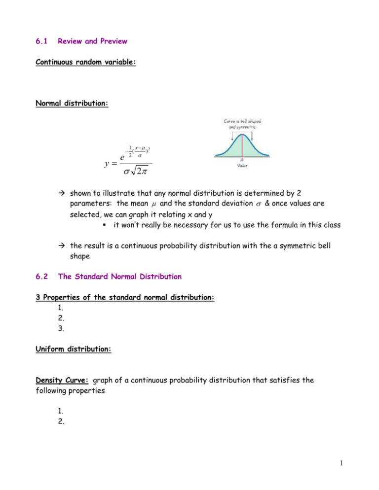
Normal distribution:
y
e
1 x 2
 (
)
2 
 2
 shown to illustrate that any normal distribution is determined by 2
parameters: the mean  and the standard deviation  & once values are
selected, we can graph it relating x and y
 it won’t really be necessary for us to use the formula in this class
 the result is a continuous probability distribution with the a symmetric bell
shape
6.2
The Standard Normal Distribution
3 Properties of the standard normal distribution:
1.
2.
3.
Uniform distribution:
Density Curve: graph of a continuous probability distribution that satisfies the
following properties
1.
2.
1
 The area of the curve becomes 1 when we make its height equal to the value of
1
range
 Because the total area under the density curve is equal to 1, there is a
correspondence between area and probability
 To find the area, multiply the width & height
 Ex: A statistics professor plans classes so carefully that the lengths of her
classes are uniformly distributed between 50.0 min and 52.0 min. Any time
between these 50.0 and 52.0 is possible & all of the possible values are equally
likely. If we randomly select one of her classes & let x be the random variable
representing the length of that class, then x has the following distribution
when graphed:
 Ex: Kim has scheduled a job interview immediately after her statistics class.
If the class runs longer than 51.5 min, she will be late for the interview.
What is the probability she will be late?
 Ex: For New York City weekday late-afternoon subway travel from Times
Square to the Mets stadium, you can take the #7 train that leaves Times
Square every five minutes. Given the subway departure schedule and the
arrival of a passenger, the waiting time is between 0 and 5 minutes and is a
uniform distribution. Find the probability that a randomly selected passenger
has a waiting time greater than 2 minutes.
2
Standard Normal Distribution:
 How to find probabilities when given z scores:
1. Use Table A-2 in Appendix A & on your formula sheets: gives the
cumulative area from the left up to a vertical line above a specific value
of z
a. Can only be used if it is a standard normal distribution
(mean of zero & standard deviation of 1)
b. One page of the table has negative z scores & the other has
positive z scores
c. Each value in the body of the table is a cumulative area from the
left up to a vertical boundary above a specific z score
d. Avoid confusion between z scores & areas:
z score: ___________________________________
_____________________________________
(leftmost column & top row of the table)
area: ______________________________________
(values in the body of the table)
e. The part of the z score denoting hundredths is found across the
top row of the table
2. Use a graphing calculator: gives area bounded on the left & bounded on
the right by vertical lines above any specific values
a. Press 2nd VARS
b. Choose 2: normal cdf(
c. Enter the two z scores separated by a comma then end the
parenthesis (left z score, right z score)
*Use -5 if you don’t have a left z-score
*Use 5 if you don’t have a right z-score
3
 Notation:
P(a < z < b)
denotes the probability that the z score is ____________
P(z > a)
denotes the probability that the z score is ____________
P(z < a)
denotes the probability that the z score is ____________
Note: The probability of getting any single exact value is zero: P(z = a) = 0
--Because the area of a single value would be a vertical line, there would
not be any area so P(a ≤ z ≤ b) = P(a < z < b)
 How to find the probability of a value less than a particular z score:
Ex #1: If thermometers have an average (mean) reading of 0 degrees and
a standard deviation of 1 degree for freezing water, and if one
thermometer is randomly selected, find the probability that, at the
freezing point of water, the reading is less than 1.58 degrees.
Ex #2: A bone mineral density test can be helpful in identifying the
presence or likelihood of osteoporosis, a disease causing bones to become
more fragile and more likely to break. The result of a bone density test is
commonly measured as a z-score. The population of z-scores is normally
distributed with a mean of 0 and a standard deviation of 1, so these test
results meet the requirements of a standard normal distribution. A
randomly selected adult undergoes a bone density test. Find the
probability that the result is a reading less than 1.27.
4
 How to find the probability of a value above a particular z score:

On the graphing calculator, use normalcdf(left z-score, right zscore) ______________________
Ex #1: Using the thermometers from the previous example, find the probability
of randomly selecting one thermometer that reads above -1.23 degrees.
Ex #2: A randomly selected adult undergoes a bone density test as
described by the previous example. Find the probability that the result is
a reading above -1.00.
5
 How to find the area between two z scores:
Ex #1: Find the probability that the chosen thermometer reads between
-2.00 degrees and 1.50 degrees.
Ex #2: A randomly selected adult undergoes a bone density test as
described by the previous example. Find the probability that the reading is
between -1.00 and -2.50.
6
 Finding z scores from known areas:
1.
2.
 Select the closest value in the table (except special cases that are used
more often)
Special Cases:
z-score
1.645
-1.645
2.575
-2.575
Above 3.49
Below -3.49
Cumulative Area
from the Left
0.9500
0.0500
0.9950
0.0050
0.9999
0.0001
 Ex #1a: Use the same thermometers as before with temperature
readings at the freezing point of water that are normally distributed with
a mean of 0ºC and a standard deviation of 1ºC. Find the temperature
corresponding to P95, the 95th percentile. (Find the temperature separating
the bottom 95% from the top 5%.
--We search for the area of 0.95 in table A-2 & then the
corresponding z score which is ___________
--So, the 95th percentile is the temperature reading of ________
--When tested at freezing, 95% of the readings will be less than or
equal to ________
7
 Ex #1b: Find the temperatures separating the bottom 2.5% and the
top 2.5%.
--Find the z score to the left for an area of 0.025
--Find the z score to the right for an area of 0.975
---
 Ex #2a: Use the previous example about the bone density tests that
are normally distributed with a mean of 0 and a standard deviation of 1, so
they meet the requirements of a standard normal distribution. Find the
bone density score corresponding to P90, the 90th percentile. That is, find
the bone density score that separates the bottom 90% from the top 10%.
 Ex #2b: Find the bone density test score that separates the bottom
5% and the score that separates the top 5%.
8
Critical Value for the standard normal distribution: a z-score separating unlikely
values from those that are likely to occur
 Notation: z denotes the z-score with an area of α to its right
o α is the Greek letter alpha
 Remember that Table A-2 lists cumulative areas to the left of a given zscore, so use 1 – α to find z
 Finding critical values will become extremely important in the next few
chapters!
 Ex #3: In the expression z , let α = 0.025 and find the value of z0.025
 Ex #4: Find the value of z0.484
9
6.3
Applications of Normal Distributions
If we convert values to standard scores using the following formula,
z
x

(round z scores to 2 decimal places)
 The area in any normal distribution bounded by some score x is the same as
the area bounded by the equivalent z score in the standard normal distribution
so you can use Table A-2
z
x

 How to find areas with a nonstandard normal distribution:
1. Sketch a normal curve, label the mean and the specific x values, then
shade the region representing the desired probability
2. For each relevant value x that is a boundary for the shaded region, use
the formula to convert that value to the equivalent z score
3. Use Table A-2 or a graphing calculator to find the area of the shaded
region. This area is the desired probability.
Ex #1: The safe load for a water taxi was found to be 3500 pounds and the mean
weight of a passenger is assumed to be 140 pounds. Let’s assume a “worst case”
scenario in which all of the passengers are adult men. Based on data from the
National Health and Nutrition Examination Survey, assume that weights of men
are normally distributed with a mean of 172 lbs and a standard deviation of 29
lbs. If one man is randomly selected, find the probability that he weighs less
than 174 pounds (the value suggested by the National Transportation and Safety
Board).
x
z

10
Ex #2: A psychologist is designing an experiment to test the
effectiveness of a new training program for airport security screeners.
She wants to begin with a homogeneous group of subjects having IQ scores
between 85 and 125. Given that IQ scores are normally distributed with a
mean of 100 and a standard deviation of 15, what percentage of people
have IQ scores between 85 and 125?
Ex #3: Women have heights that are normally distributed with a mean of
63.8 inches and a standard deviation of 2.6 inches. What percent of women
are at least 70 inches tall?
11
Ex #4: British Airways and many other airlines have a requirement that a
member of the cabin crew must have a height between 62 and 73 inches (or
between 5 ft 2 in and 6 ft 1 in). Given that men have normally distributed
heights with a mean of 69.5 in. and a standard deviation of 2.4 in., find the
percentage of men who satisfy the height requirement.
 How to find values from known areas or probabilities:
1. Sketch a normal distribution curve, enter the given probability or
percentage in the appropriate region of the graph, and identify the x
value(s) that you’re looking for.
2. Refer to the body of table A-2 to find the closest area to the left of x
& then identify the corresponding z score
3. Use the following form of the z score formula to solve for x:
x    (z   )
4. Refer to the sketch of the curve to verify that the solution makes
sense in the context of the graph and the context of the problem.
Helpful Hints:
a. Don’t confuse z-scores & areas. Z-scores are distances along the
horizontal scale, but areas are regions under the normal curve.
b. Choose the correct (left/right) side of the graph. A value separating
the top 10% from the others will be on the right side. A value separating
the bottom 10% will be located on the left side.
12
c. A z-score must be negative if it’s located on the left half of the normal
distribution.
d. Areas (or probabilities) are positive or zero values, but they are never
negative.
Ex #5: In a previous example, we found that 52.79% of men have weights
less than the value of 174 lbs set by the National Transportation and
Safety Board. What weight separates the lightest 99.5% of men from the
heaviest 0.5%? Again, assume the weights of men are normally distributed
with a mean of 172 lbs and a standard deviation of 29 lbs.
Ex #6: When designing an environment, one common criterion is to use a
design that accommodates 95% of the population. What aircraft ceiling
height will allow 95% of men to stand without bumping their heads? That
is, find the 95th percentile of heights of men. Assume that heights of men
are normally distributed with a mean of 69.5 inches and a standard
deviation of 2.4 inches.
13
Ex #7: When designing the placement of a CD player in a new model car,
engineers must first consider the forward grip reach, the driver must not
move his or her body in a way that could be distracting and dangerous.
Design engineers decide that the CD player should be placed so that it is
within the forward grip reach of 95% of women. Women have forward grip
reaches that are normally distributed with a mean of 27.0 in and a
standard deviation of 1.3 in. Find the forward grip reach of women that
separates the longest 95% from the others.
Ex #8: Some educators argue that all students are served better if they
are separated into groups according to their abilities. Assume that
students are to be separated into a group with IQ scores in the bottom
30%, a second group with IQ scores in the middle 40%, and a third group
with IQ scores in the top 30%. The Wechsler Adult Intelligence Scale
yields an IQ score obtained through a test, and the scores are normally
distributed with a mean of 100 and a standard deviation of 15. Find the
Wechsler IQ scores that separate the 3 groups.
 How to use the graphing calculator to find the area between two values:
1. Press 2nd VARS
2. Choose 2: normalcdf(
3. Enter the two values, the mean, and the standard deviation separated by
commas (left value, right value, mean, standard deviation)
14
 How to use the graphing calculator to find a value corresponding to a known
area:
1. Press 2nd VARS
2. Choose 3: invNorm(
3. Enter the total area to the left of the value, the mean, and the standard
deviation (total area to the left, mean, standard deviation)
Use the graphing calculator to answer examples 4 and 8:
Ex #4: British Airways and many other airlines have a requirement that a
member of the cabin crew must have a height between 62 and 73 inches (or
between 5 ft 2 in and 6 ft 1 in). Given that men have normally distributed
heights with a mean of 69.5 in. and a standard deviation of 2.4 in., find the
percentage of men who satisfy the height requirement.
Ex #8: Some educators argue that all students are served better if they
are separated into groups according to their abilities. Assume that
students are to be separated into a group with IQ scores in the bottom
30%, a second group with IQ scores in the middle 40%, and a third group
with IQ scores in the top 30%. The Wechsler Adult Intelligence Scale
yields an IQ score obtained through a test, and the scores are normally
distributed with a mean of 100 and a standard deviation of 15. Find the
Wechsler IQ scores that separate the 3 groups.
.
15
When
1.
2.
3.
4.
dealing with normal distributions, always remember…
Draw a graph to visualize the information
Determine whether we want to find an area or a value of x
We usually work with a cumulative area from the left
Z score and x values are distances along horizontal scales, but percentages or
probabilities correspond to areas under a curve
16
6.4
Sampling Distributions & Estimators
Sampling distribution of a statistic:
 such as a sample mean or sample proportion
 typically represented as a probability distribution in the form of a table,
probability histogram, or formula
Sampling Distribution of the Sample Mean:
 typically represented as a probability distribution in the form of a table,
probability histogram, or formula
 Ex #1: A friend has three children with ages 1, 2, and 5. Note that the mean
of this population is 8/3.
a.
If two ages are randomly selected with replacement from the population
{1,2,5}, identify the sampling distribution of the sample mean by creating
a table representing the probability distribution of the sample mean.
Sample
Mean ( x )
Probability
b. Find the mean of the sampling distribution:
Because the above table is a probability distribution, we can use the
following formula:   [ x  P( x)]
17
c. The population mean is 8/3. Do the sample means target the value of the
population mean?
 Behavior of Sample Means:
o The sample means target the value of the population mean
o The distribution of sample means tends to be a normal distribution
(tends to become closer to a normal distribution as sample size
increases)
 Ex #2: Look at the following example about rolling a die 5 times and finding
the mean x of the results that are generated as this process continues
indefinitely.
Sampling Distribution of the Sample Variance:
 typically represented as a probability distribution in the form of a table,
probability histogram, or formula
 Be sure to use the correct computations for standard deviations or variances
depending on whether you have a population or sample
18
o Population standard deviation:  
o Sample standard deviation: s 
o Population variance: 
o Sample variance: s 2 
2
 (x  )
N
 ( x  x)
 (x  )

2
2
n 1
2
N
 (x  )
2
n 1
 Behavior of Sample Variances:
o Sample variances target the value of the population variance (ie: the
mean of the sample variances is the population variance)
o The distribution of sample variances tends to be a distribution skewed
to the right.
 Ex #3: Look at the following example about rolling a die 5 times and finding
the variance s2 of the results that are generated as this process continues
indefinitely.
19
Sampling distribution of the sample proportion:
 Notation:
o p = population proportion
o
p = sample proportion
 Ex #4: Look at the following example about rolling a die 5 times and finding
the sample proportions that are generated as this process continues
indefinitely.
 Behavior of Sample Proportions:
o Sample proportions target the value of the population proportion (ie:
the mean of the sample proportions is the population proportion)
o The distribution of sample proportions tends to approximate a normal
distribution
 Ex #5: When 2 births are randomly selected, the sample space is ________
__________. The four equally likely outcomes suggest that the probability
of no girls is _____. The following display shows the probability distribution
for the number of girls, then a table and graph describing the sampling
distribution for the proportion of girls.
20
 Ex #6: A quarterback threw 1 interception in his 1st game, 2 interceptions in
his 2nd game, and 5 interceptions in his 3rd game and then he retired. Consider
the population consisting of the values 1, 2, and 5. Notice that the proportion
of odd numbers in the population is 2/3.
a. List all of the different possible samples of size n = 2 selected with
replacement. For each sample, find the proportion of numbers that are
odd. Use a table to represent the sampling distribution for the
proportion of odd numbers.
Sample
Proportion of
Odd Numbers
Probability
b. Find the mean of the sampling distribution for the proportion of odd
numbers:
Proportion of
Odd Numbers
Probability
Because it’s a probability distribution, we can
use the following formula:   [ x  P( x)]
c. For the population of 1, 2, and 5, the proportion of odd numbers is
2/3. Is the mean of the sampling distribution for the proportion of odd
numbers also equal to 2/3? Do sample proportions target the value of
the population proportion? That is, do the sample proportions have a
mean that is equal to the population proportion?
21
Estimator: A statistic used to infer (estimate) the value of a population parameter
Unbiased Estimators: a statistic that targets the value of the population parameter in
the sense that the sampling distribution of the statistic has a mean that is equal to the
mean of the corresponding parameter.
 Ex: ________________________________________________
Biased Estimators: a statistic that does NOT target the value of the corresponding
population parameter.
 Ex: _________________________________________________
 s is still often used to estimate  because the bias is relatively small in large
samples
 Sample range and median should never be used to estimate population range
and median
Ex: List all of the different possible samples of size n = 2 selected from
the previous set: {1,2,5} with replacement. For each sample, find the
range. Use a table to represent the sampling distribution for the range.
Sample
Range
Probability
1, 1
1/9
1, 2
1/9
1, 5
1/9
2, 1
1/9
2, 2
1/9
2, 5
1/9
5, 1
1/9
5, 2
1/9
5, 5
1/9
The mean of the sample ranges =
The population range =
22
Why sample with replacement?
 When selecting a relatively small sample from a large population, it makes no
significant difference whether we sample with or without replacement
 Sampling with replacement results in independent events that are unaffected
by previous outcomes, and independent events are easier to analyze and they
result in simpler formulas
23
6.5
The Central Limit Theorem
Central Limit Theorem:
 Practical Rules Commonly Used:
1. If the original population is not itself normally distributed (uniform, skewed,
etc.) & you have samples of size n greater than 30, the distribution of the
sample means can be approximated reasonably well by a normal distribution.
The approximation gets better as the sample size n increases.
2. If the original population is itself normally distributed, then the sample means
will be normally distributed for ANY sample size n (not just the values of n
larger than 30)
3. If the original population is not itself normally distributed and n ≤ 30, then the
distribution of the sample mean cannot be approximated by a normal
distribution and you cannot use the central limit theorem.
Mean of all values of
Standard deviation of all values of
z-score conversion of
x = µ
x:
x:
x:
x =  / n
z
x

n
 When Should I Use the Central Limit Theorem?
1. Does the original population have a normal distribution or is n > 30?

If yes, ____________________________________________

If not, ____________________________________________
24
2. Are you using a normal distribution with a single value x or the mean
sample of n values?

x
from a
If it’s an individual value from a normally distributed population, use what
xx
we learned in section 6.3 and find the z-score using the formula: z 


If it’s a mean from some sample of n values, use the central limit theorem
x
to find the z-score using the formula: z 

n
 Two Different Distributions:
1. the distribution of the original population -- _________________________
2. the distribution of the sample means -- _____________________________

x
is often called the _______________________________
 Ex #1: Computers are often used to randomly generate digits of telephone
numbers to be called for polling purposes. The digits 0, 1, 2, 3, 4, 5, 6, 7, 8, 9 are
generated in such a way that they are all equally likely. The first graph shows the
histogram of 500,000 generated digits (which appears to be a uniform
distribution).
 When the 500,000 digits are grouped into 5,000 samples with each sample
have n = 100 values, the mean for each sample of the 5,000 sample means are
shown in the second graph.
 Even though the original 500,000 digits have a uniform distribution, the
distribution of the 5,000 sample means is approximately a normal distribution.
25
 Ex #2: When designing elevators, an obviously important consideration is the
weight capacity. An Ohio college student died when he tried to escape from a
dormitory elevator that was overloaded with 24 passengers. The elevator was
rated for a capacity of 16 passengers with a total weight of 2500 lbs.
Weights of adults are changing over time and the following table shows the
values of recent parameters. For the following, we assume a worst-case
scenario in which all of the passengers are males (which could easily happen in
a dormitory setting). If an elevator is loaded to a capacity of 2500 lb with 16
males, the mean weight of a passenger is 156.25 lb.
Males
Females
µ
182.9 lb
165.0 lb
σ
40.8 lb
45.6 lb
Distribution
Normal
Normal
a. Find the probability that 1 randomly selected adult male has a weight
greater than 156.25 lb.
b. Find the probability that a sample of 16 randomly selected adult males has
a mean weight greater than 156.25 lb (so that the total weight exceeds the
maximum capacity of 2500 lb)
26
Ex #3: Men are typically heavier than women and children, so when loading a
water taxi, let’s assume a worst case scenario in which all passengers are men.
Based on data from the National Health & Nutrition Examination Survey,
assume that weights of men are normally distributed with a mean of 172 lbs.
and a standard deviation of 29 lbs.
a. Find the probability that if an individual man is randomly selected, his
weight will be greater than 175 lbs.
b. Find the probability that 20 randomly selected men will have a mean
that is greater than 175 lbs. (so that their total weight exceeds the
safe capacity of 3500 lbs.)
 These types of calculations are used by engineers when designing ski lifts,
elevators, escalators, airplanes, …
27
 Interpreting Results of the Central Limit Theorem:
 Rare Event Rule: If, under a given assumption, the probability of a particular
observed event is exceptionally small, we conclude that the assumption is
_____________________________________.
 Ex #4: Assume that the population of human body temperatures has a mean
of 98.6ºF (as is commonly believed). Also assume that the population standard
deviation is 0.62ºF (based on data from University of Maryland researchers).
If a sample size n = 106 is randomly selected, find the probability of getting a
mean of 98.2ºF or lower.
 Ex #5: Cans of regular Coke are labeled to indicate that they contain 12 oz.
Data Set 19 in Appendix B lists measured amounts for a sample of Coke cans. The
corresponding sample statistics are n = 36, x = 12.19 oz. Assuming that the Coke
cans are filled so that µ = 12 oz (as labeled) and the population standard deviation
is σ = 0.11 oz (based on the sample results). Find the probability that a sample of
36 cans will have a mean of 12.19 oz or greater. Do these results suggest that
the Coke cans are filled with an amount greater than 12.00 oz?
28
 Correction for a Finite Population:
 When sampling without replacement and the sample size n is greater than 5%
of the finite population size N (that is, n > 0.05N), adjust the standard
deviation of the sample means
 x by multiplying it by
the finite population correction factor:
N n
N 1
 For most of our examples, we are sampling with replacement or the population
is infinite or the sample size does not exceed 5% of the population size, so the
correction factor DOES NOT APPLY.
29
6.6
Assessing Normality
This section provides criteria for determining whether the requirement of a normal
distribution is satisfied.
 Visual inspection of a histogram: see if it is roughly bell-shaped & identify any
outliers
 Construct a new graph called a normal quantile plot
Normal quantile plot (or normal probability plot):
 If the points do NOT lie close to a straight line or the points exhibit some
pattern that is NOT a straight-line pattern, then the data appear to come
from a population that does NOT have a normal distribution
 If the pattern of the points is reasonably close to a straight line, then the
data appear to come from a population that has a normal distribution
In this course, you will not be required to construct normal quantile plots but should
understand what they are.
30
6.7
Normal as Approximation to Binomial
Normal Distribution as Approximation to Binomial Distribution:


 Procedure:
1. Check the requirement that np ≥ 5 and nq ≥ 5
2. Find the values of the parameter by calculating
  np and   npq
3. Identify the discrete value x (the number of successes). Change the
discrete value x by replacing it with the interval from (x – 0.5) to (x +
0.5)
4. Draw a normal curve and enter the values of  ,  , and replace x with
either (x – 0.5) to (x + 0.5), as appropriate
5. Find the area corresponding to the desired probability by first finding
xx
the z score z 
, use that z score to find the area to the left of

the adjusted value of x, and find the desired probability
 Ex #1: An American Airlines Boeing 767-300 aircraft has 213 seats. When
fully loaded with passengers, baggage, cargo, & fuel, the pilot must verify that
the gross weight is below the maximum allowable limit, and the weight must be
properly distributed so that the balance of the aircraft is within safe
acceptable limits. Instead of weighing each passenger, their weights are
estimated according to Federal Aviation Administration rules. In reality, we
know that men have a mean weight of 172 lbs. and women have a mean weight
of 143 lbs, so disproportionately more male passengers may result in an unsafe
overweight situation. Assume that if there are at least 122 men in a roster of
213 passengers, the load must be somehow adjusted. Assuming that
passengers are booked randomly, male passengers and female passengers are
equally likely, and the aircraft is full of adults, find the probability that a
Boeing 767-300 with 213 passengers has at least 122 men.
n=
2 categories:
P(male) =
31
1. np
nq
2.
  np
  npq
3. We want the probability of “at least 122 males” so we adjust the x value
of 122 by using the continuity correction factor:
4. We want the area representing the region bounded by
5. Convert 121.5 to a z score z 
xx

Use table A-2 to find the area to the left of _____ = _________
The probability of having at least 122 men out of 213 adult
passengers is ___________________
 Ex #2: In 431 NFL football games that went to overtime, the teams that won
the coin toss went on to win 235 of those games. If the coin-toss method is
fair, we expect that the teams winning the coin toss would win about 50% of
the games, so we expect about 215.5 wins in 431 overtime games. Assuming
that there is a 0.5 probability of winning a game after winning the coin toss,
find the probability of getting at least 235 winning games among the 431
teams that won the coin toss. That is, given n = 431 and p = 0.5, find P(at least
235 wins).
1. np =
nq =
2.
  np =
  npq =
32
3. We want the probability of “at least 235 wins” so we adjust the x value
of 235 by using the continuity correction factor:
4. We want the area representing the region bounded by
5. Convert 234.5 to a z score z 
xx

Use table A-2 to find the area to the left of ______ = _________
The probability of having at least 235 wins out of 431 is
*
 Continuity Corrections: When we use the normal distribution (which is a
continuous probability distribution) as an approximation to the binomial
distribution (which is discrete),
 Procedure:
1. When using the normal distribution as an approximation to the binomial
distribution, ALWAYS use the continuity correction.
2. First, identify the discrete whole number x that is relevant to the binomial
probability problem. Then figure out if you want at least x, more than x,
fewer than x, …
3. Draw a normal distribution centered about
 , then draw a vertical strip area
centered over x. Mark the left side of the strip with the number equal to (x –
0.5) and the right side of the strip with (x + 0.5). Consider the entire area of
the strip to represent the probability of the discrete whole number x itself.
4. Determine whether the value of x itself should be included in the probability
you want (ex: “at least x” does include x & “more than x” does not include x).
Shade the area to the right or left of the strip, as appropriate & also the
interior of the strip if and only if x itself is to be included. This total shaded
region corresponds to the probability you’re looking for.
33
Example list of continuity corrections:
Statement
Area
At least 122
(includes 122 and above)
More than 122
(doesn’t include 122)
At most 122
(includes 122 and below)
Fewer than 122
(doesn’t include 122)
Exactly 122
 Ex: A recent survey showed that among 2013 randomly selected adults, 1358
(or 67.5%) stated that they are Internet users (based on data from Pew
Research Center). If the proportion of all adults using the Internet is
actually 2/3, find the probability that a random sample of 2013 adults will
result in exactly 1358 users.
n=
x=
p=
q=
1. Verify that we can use a normal distribution:
np
nq
2.   np
  npq
34
3. We want the probability of “exactly 1358 Internet users” so we adjust
the x value of 122 by using the continuity correction factor:
4. We want the area representing the region bounded by _____________
____________________
5. Convert 1358.5 to a z score z 
xx

Use table A-2 to find the area to the left of ______ = _________
Convert 1357.5 to a z score z 
xx

Use table A-2 to find the area to the left of ______ = ________
The area we want is between these two values so find the difference:
If we assume that 2/3 of all adults use the Internet, the probability of
getting exactly 1358 Internet users among 2013 randomly selected
people is ___________
*
 Calculation errors: If you use a graphing calculator to determine the
probabilities, the numbers may be off due to …
1. The use of the normal distribution results in an approximate value that
is the area of the shaded region, whereas the exact correct area is a
rectangle above 1358.
2. The use of table A-2 forced us to find one of a limited number of table
values based on a rounded z score.
35
 Interpreting Results:
Using probabilities to determine when results are unusual:
Unusually high: x successes among n trials is an unusually high number of
successes if ________________________________________
Unusually low: x successes among n trials is an unusually low number of
successes if ________________________________________
36