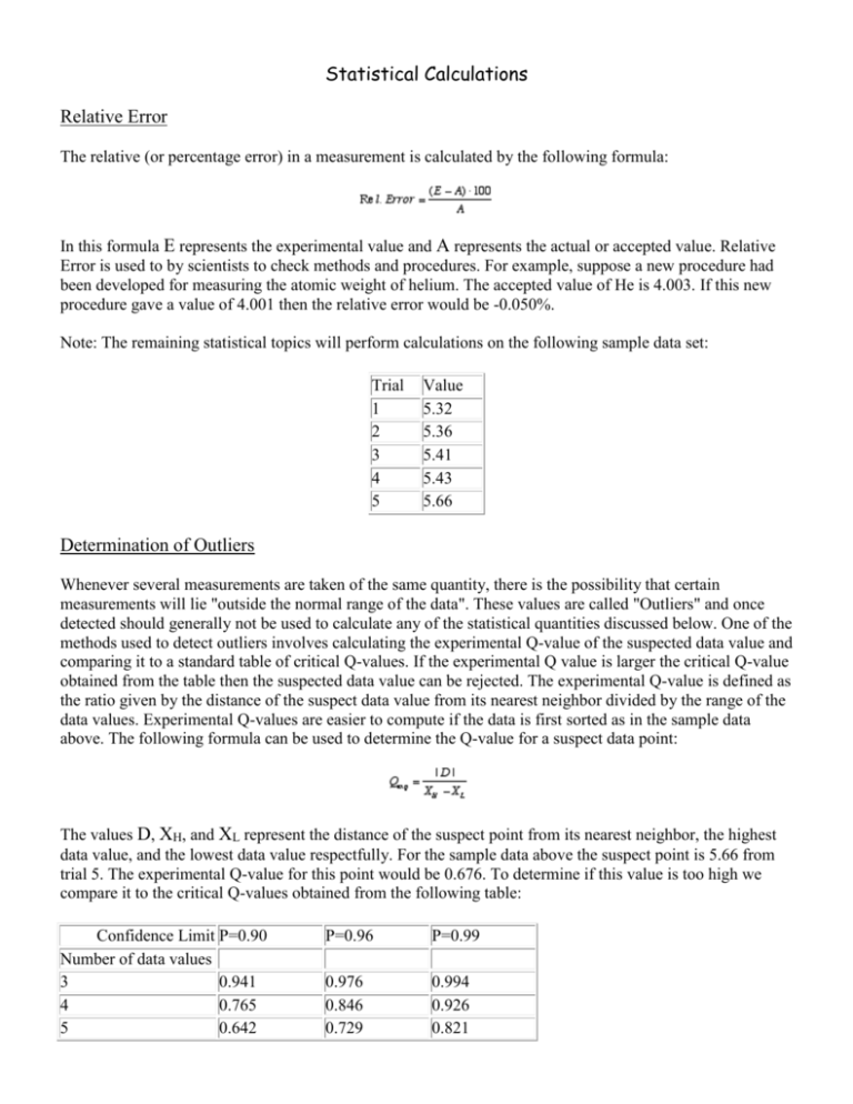
Statistical Calculations
Relative Error
The relative (or percentage error) in a measurement is calculated by the following formula:
In this formula E represents the experimental value and A represents the actual or accepted value. Relative
Error is used to by scientists to check methods and procedures. For example, suppose a new procedure had
been developed for measuring the atomic weight of helium. The accepted value of He is 4.003. If this new
procedure gave a value of 4.001 then the relative error would be -0.050%.
Note: The remaining statistical topics will perform calculations on the following sample data set:
Trial
1
2
3
4
5
Value
5.32
5.36
5.41
5.43
5.66
Determination of Outliers
Whenever several measurements are taken of the same quantity, there is the possibility that certain
measurements will lie "outside the normal range of the data". These values are called "Outliers" and once
detected should generally not be used to calculate any of the statistical quantities discussed below. One of the
methods used to detect outliers involves calculating the experimental Q-value of the suspected data value and
comparing it to a standard table of critical Q-values. If the experimental Q value is larger the critical Q-value
obtained from the table then the suspected data value can be rejected. The experimental Q-value is defined as
the ratio given by the distance of the suspect data value from its nearest neighbor divided by the range of the
data values. Experimental Q-values are easier to compute if the data is first sorted as in the sample data
above. The following formula can be used to determine the Q-value for a suspect data point:
The values D, XH, and XL represent the distance of the suspect point from its nearest neighbor, the highest
data value, and the lowest data value respectfully. For the sample data above the suspect point is 5.66 from
trial 5. The experimental Q-value for this point would be 0.676. To determine if this value is too high we
compare it to the critical Q-values obtained from the following table:
Confidence Limit P=0.90
Number of data values
3
0.941
4
0.765
5
0.642
P=0.96
P=0.99
0.976
0.846
0.729
0.994
0.926
0.821
6
7
8
9
10
11
12
13
14
15
16
17
18
19
20
21
22
23
24
25
26
27
28
29
30
0.560
0.507
0.468
0.437
0.412
0.542
0.522
0.503
0.488
0.475
0.463
0.452
0.442
0.433
0.425
0.418
0.411
0.404
0.399
0.393
0.388
0.384
0.380
0.376
0.372
0.644
0.586
0.543
0.510
0.483
0.460
0.441
0.425
0.411
0.399
0.388
0.379
0.370
0.363
0.356
0.350
0.344
0.338
0.333
0.329
0.324
0.320
0.316
0.312
0.309
0.740
0.680
0.634
0.598
0.568
0.392
0.376
0.361
0.349
0.338
0.329
0.320
0.313
0.306
0.300
0.295
0.290
0.285
0.281
0.277
0.273
0.269
0.266
0.263
0.260
For a confidence limit of 90% (P=0.90) trial 5 can be rejected since its experimental Q-value (0.676) is larger
than the critical Q-value for 5 trials (0.642). However, the value could not be rejected if one desired a higher
confidence limit since the experimental Q-value is less than the corresponding critical Q-value at the higher
confidence limits.
Note: The following statistical calculations are going to be done at a confidence limit of 90% (P=0.90) and
since trial 5 has been determined to be an "outlier" at this confidence limit it will be rejected from those
statistical calculations.
Mean or Average
The mean of a set of values, which is denoted by the symbol x, is calculated by the following formula:
In this formula n represents the number of data points, and xi represents a specific data value. Applying this
formula to the sample data above one obtains a mean of 5.380. (If trial 5 is not rejected the mean would be
5.436.)
Median
The median value of a series of measurements is the middle value. In order to find the median of a set of
values the measurements must be sorted as the sample data above is. The median of the sample data is the
value of trial 3 if trial 5 is not being rejected, that is, 5.41. If the median is being determined for an even
number of trials the average of the two middle values can be taken. Since we are rejecting trial 5 the median
would be the average of trials 2 and 3 which is 5.39.
Standard Deviation
The standard deviation, sometimes abbreviated with the Greek symbol sigma (s), gives an indication of how
well the data is grouped around the mean value. A large standard deviation indicates that several values were
significantly above and below the mean indicating low precision data, while a small standard deviation
indicates that the values were quite close to the mean indicating high precision data. For example, both plots
below show the results of two procedures, both of which attempted to measure the atomic weight of Ne.
Both plots have a mean of 10, however, the data from procedure 1 is of higher precision because the standard
deviation is only 1.61 vs. 2.45 for procedure 2.
The formula for calculating the standard deviation is given below:
When this formula is applied to the above sample data a standard deviation of 0.050 is obtained to a
confidence limit of 90%. This means that 68% of the values lie within ±0.050 units of the mean or within the
range of 5.330 to 5.430 (5.380 ± 0.050) for the above sample data. Plus or minus two standard deviations
(5.380 ± 0.100) of the mean encloses about 98% of all data points.
Average Deviation
The average deviation is easier to compute but less often used than the standard deviation. It is computed by
the following formula:
In terms of the error curve the probability that another measurement lies within ±a of the mean is 57%. For
the sample data given above the average deviation would be 0.04. This means that the probability of the next
measurement falling in the range of 5.34 to 5.42 (5.38 ±0.04) would be 57%.