Contingency Tables
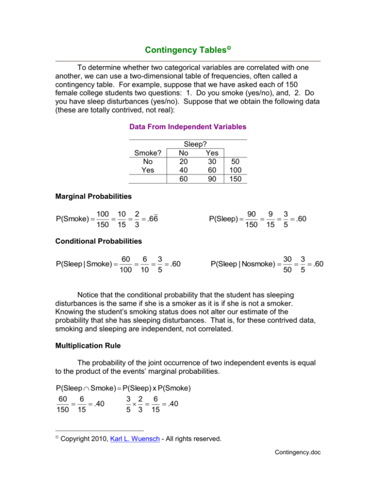
To determine whether two categorical variables are correlated with one
another, we can use a two-dimensional table of frequencies, often called a
contingency table. For example, suppose that we have asked each of 150
female college students two questions: 1. Do you smoke (yes/no), and, 2. Do
you have sleep disturbances (yes/no). Suppose that we obtain the following data
(these are totally contrived, not real):
Data From Independent Variables
Smoke?
No
Yes
Sleep?
No
Yes
20
30
40
60
60
90
50
100
150
Marginal Probabilities
P(Smoke) 
100 10 2

  .66
150 15 3
P(Sleep) 
90
9 3

  .60
150 15 5
Conditional Probabilities
P(Sleep | Smoke) 
60
6 3

  .60
100 10 5
P(Sleep | Nosmoke) 
30 3
  .60
50 5
Notice that the conditional probability that the student has sleeping
disturbances is the same if she is a smoker as it is if she is not a smoker.
Knowing the student’s smoking status does not alter our estimate of the
probability that she has sleeping disturbances. That is, for these contrived data,
smoking and sleeping are independent, not correlated.
Multiplication Rule
The probability of the joint occurrence of two independent events is equal
to the product of the events’ marginal probabilities.
P(Sleep  Smoke)  P(Sleep) x P(Smoke)
60
6
3 2
6

 .40
 
 .40
150 15
5 3 15

Copyright 2010, Karl L. Wuensch - All rights reserved.
Contingency.doc
2
Addition Rule
Suppose that the probability distribution for final grades in PSYC 2101
were as follows:
Grade
Probability
A
.2
B
.3
C
.3
D
.15
F
.05
The probability that a randomly selected student would get an A or a B,
P(A  B)  P(A)  P(B)  .2  .3  .5 , since A and B are mutually exclusive events.
Now, consider our contingency table, and suppose that the “sleep”
question was not about having sleep disturbances, but rather about “sleeping”
with men (that is, being sexually active). Suppose that a fundamentalist preacher
has told you that women who smoke go to Hades, and women who “sleep” go
there too. What is the probability that a randomly selected woman from our
sample is headed to Hades? If we were to apply the addition rule as we did
9 10 19


 1.27 , but a probability cannot
earlier, P(Sleep)  P(Smoke) 
15 15 15
exceed 1, something is wrong here. The problem is that the events (sleeping
and smoking) are not mutually exclusive, so we have counted the overlap
between sleeping and smoking (the 60 women who do both) twice. We need to
subtract out that double counting. If we look back at the cell counts, we see that
30 + 40 + 60 = 130 of the women sleep and/or smoke, so the probability we seek
must be 130/150 = 13/15 = .87. Using the more general form of the addition rule,
9 10 6 13
P(Sleep  Smoke)  P(Sleep)  P(Smoke) - P(Sleep  Smoke) 


 .87.
15 15 15 15
Data From Correlated Variables
Now, suppose that the “smoke” question concerned marijuana use, and
the “sleep” question concerned sexual activity, variables known to be related.
Smoke?
No
Yes
Sleep?
No
Yes
30
20
40
60
70
80
50
100
150
Marginal Probabilities
P(Smoke) 
100 2
  .6 6
150 3
P(Sleep) 
80
8

 .5 3
150 15
3
Conditional Probabilities
P(Sleep | Smoke) 
60
6 3

  .60
100 10 5
P(Sleep | Nosmoke) 
20 2
  .40
50 5
Now our estimate of the probability that a randomly selected student
“sleeps” depends on what we know about her smoking behavior. If we know
nothing about her smoking behavior, our estimate is about 53%. If we know she
smokes, our estimate is 60%. If we know she does not smoke, our estimate is
40%. We conclude that the two variables are correlated, that female students
who smoke marijuana are more likely to be sexually active than are those who do
not smoke.
Multiplication Rule
If we attempt to apply the multiplication rule to obtain the probability that a
randomly selected student both sleeps and smokes, using the same method we
employed with independent variables, we obtain:
8 2 16
P(Sleep  Smoke)  P(Sleep) x P(Smoke) 
 
 .3 5 . This answer is,
15 3 45
however, incorrect. Sixty of 150 students are smoking sleepers, so we should
have obtained a probability of 6/15 = .40. The fact that the simple form of the
multiplication rule (the one which assumes independence) did not produce the
correct solution shows us that the two variables are not independent.
If we apply the more general form of the multiplication rule, the one which
does not assume independence, we get the correct solution:
2 3 6
P(Smoke  Sleep)  P(Smoke)  P(Sleep | Smoke)   
 .40.
3 5 15
Real Data
Finally, here is an example using data obtained by Castellow, Wuensch,
and Moore (1990, Journal of Social Behavior and Personality, 5, 547-562). We
manipulated the physical attractiveness of the plaintiff and the defendant in a
mock trial. The plaintiff was a young women suing her male boss for sexual
harassment. Our earlier research had indicated that physical attractiveness is an
asset for defendants in criminal trials (juries treat physically attractive defendants
better than physically unattractive defendants), and we expected physical
attractiveness to be an asset in civil cases as well. Here are the data relevant to
the effect of the attractiveness of the plaintiff.
4
Attractive?
No
Yes
Guilty?
No
Yes
33
39
17
56
50
95
72
73
145
Guilty verdicts (finding in favor of the plaintiff) were more likely when the
plaintiff was physically attractive (the conditional probability is 56/73 = 77%) than
when she was not physically attractive (the conditional probability is 39/72 =
54%). There are advantages to using odds rather than probabilities. When the
plaintiff was physically attractive the odds of a guilty verdict were 56/17 = 3.294 –
a guilty verdict was 3.294 times more likely than a not guilty verdict. When the
plaintiff was not physically attractive the odds of a guilty verdict were 39/33 =
1.182 – a guilty verdict was 1.182 times more likely than a not guilty verdict.
The magnitude of the effect of physical attractiveness can be obtained by
computing an odds ratio. For these data the odds ratio is 3.294/1.182 = 2.79 –
that is, when the plaintiff was attractive, the odds of a guilty verdict were 2.79
times higher than when the plaintiff was not attractive.
We also found that physical attractiveness was an asset to the defendant.
Here are the data:
Attractive?
No
Yes
Guilty?
No
Yes
17
53
33
42
50
95
70
75
145
Guilty verdicts (finding in favor of the plaintiff) were less likely when
the defendant was physically attractive (42/75 = 56%) than when he was not
53 / 17
physically attractive (53/70 = 76%). The odds ratio here is
 2.50.
42 / 33
If we consider the combined effects of physical attractiveness of both
litigants, guilty verdicts were most likely when the plaintiff was attractive and the
defendant was not, in which case 83% of the jurors recommended a guilty
verdict. When the defendant was attractive but the plaintiff was not, only 41% of
the jurors recommended a guilty verdict (and only 26% of the male jurors did).
83 / 17
That produces and odds ratio of
 7.03. Clearly, it is to one’s advantage
41/ 59
to appear physically attractive when in court.
5
Why Odds Ratios Rather Than Probability Ratios?
Odds ratios are my favorite way to describe the strength of the relationship
between two dichotomous variables. One could use probability ratios, but there
are problems with probability ratios, which I illustrate here.
Suppose that we randomly assign 200 ill patients to two groups. One
group is treated with a modern antibiotic. The other group gets a homeopathic
preparation. At the end of two weeks we blindly determine whether or not there
has been a substantial remission of symptoms of the illness. The data are
presented in the table below.
Remission
of
Symptoms
Treatment
No Yes
Antibiotic
10
90 100
Homeopathic 60
40 100
70 130 200
Odds of Success
For the group receiving the antibiotic, the odds of success (remission of
symptoms) are 90/10 = 9. For the group receiving the homeopathic preparation
the odds of success are 40/60 = 2/3 or about .67. The odds ratio reflecting the
strength of the relationship is 9 divided by 2/3 = 13.5. That is, the odds of
success for those treated with the antibiotic are 13.5 times higher than for those
treated with the homeopathic preparation.
Odds of Failure
For the group receiving the homeopathic preparation, the odds of failure
(no remission of symptoms) are 60/40 = 1.5. For those receiving the antibiotic
the odds of failure are 10/90 = 1/9. The odds ratio is 1.5 divided by 1/9 = 13.5.
Notice that this ratio is the same as that obtained when we used odds of
success, as, IMHO, it should be.
Now let us see what happens if we use probability ratios.
Probability of Success
For the group receiving the antibiotic, the probability of success is 90/100
= .9. For the homeopathic group the probability of success is 40/100 = .4. The
ratio of these probabilities is .9/.4 = 2.25. The probability of success for the
antibiotic group is 2.25 times that of the homeopathic group.
6
Probability of Failure
For the group receiving the homeopathic preparation the probability of
failure is 60/100 = .6. For the antibiotic group it is 10/100 = .10. The probability
ratio is .6/.1 = 6. The probability of failure for the homeopathic group is six times
that for the antibiotic group.
The Problem
With probability ratios the value you get to describe the strength of the
relationship when you compare (A given B) to (A given not B) is not the same as
what you get when you compare (not A given B) to (not A given not B). This is,
IMHO, a big problem. There is no such problem with odds ratios.
Another Example
According to a report provided by Medscape, among the general
population in the US, the incidence of narcissistic personality disorder is 0.5%.
Among members of the US Military it is 20%.
Probability of NPD.
The probability that a randomly selected member of the military will have
NPD is 20%, the probability that a randomly selected member of the general
population will have NPD is 0.5%. This yields a probability ratio of .20/.005 = 40.
Probability of NOT NPD.
The probability that a randomly selected member of the general population
will not have NPD is .995. The probability that a randomly selected member of
the military will not have NPD is .80. This yields a probability ratio of .995/.8 =
1.24.
Odds of NPD
For members of the military, .2/.8 = .25. For members of the general
population, .005/.995 = .005. The odds ratio is (.2/.8) / (.005/.995) = 49.75.
Odds of NOT NPD.
For members of the military, .8/.2 = 4. For members of the general
population, .995/.005 = 199. The odds ratio is (.995/.005) / (.8/.2) = 49.75.
Copyright 2010, Karl L. Wuensch - All rights reserved.