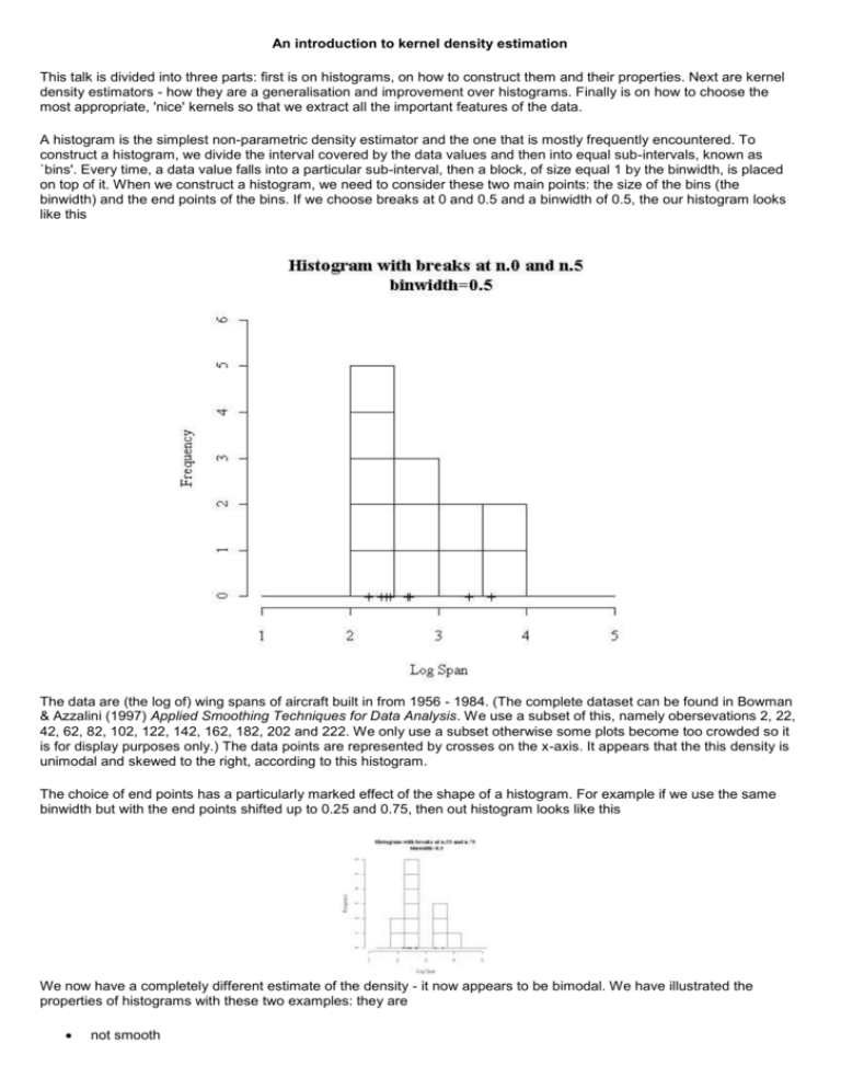
An introduction to kernel density estimation
This talk is divided into three parts: first is on histograms, on how to construct them and their properties. Next are kernel
density estimators - how they are a generalisation and improvement over histograms. Finally is on how to choose the
most appropriate, 'nice' kernels so that we extract all the important features of the data.
A histogram is the simplest non-parametric density estimator and the one that is mostly frequently encountered. To
construct a histogram, we divide the interval covered by the data values and then into equal sub-intervals, known as
`bins'. Every time, a data value falls into a particular sub-interval, then a block, of size equal 1 by the binwidth, is placed
on top of it. When we construct a histogram, we need to consider these two main points: the size of the bins (the
binwidth) and the end points of the bins. If we choose breaks at 0 and 0.5 and a binwidth of 0.5, the our histogram looks
like this
The data are (the log of) wing spans of aircraft built in from 1956 - 1984. (The complete dataset can be found in Bowman
& Azzalini (1997) Applied Smoothing Techniques for Data Analysis. We use a subset of this, namely obersevations 2, 22,
42, 62, 82, 102, 122, 142, 162, 182, 202 and 222. We only use a subset otherwise some plots become too crowded so it
is for display purposes only.) The data points are represented by crosses on the x-axis. It appears that the this density is
unimodal and skewed to the right, according to this histogram.
The choice of end points has a particularly marked effect of the shape of a histogram. For example if we use the same
binwidth but with the end points shifted up to 0.25 and 0.75, then out histogram looks like this
We now have a completely different estimate of the density - it now appears to be bimodal. We have illustrated the
properties of histograms with these two examples: they are

not smooth


depend on end points of bins
depend on width of bins
We can alleviate the first two problems by using kernel density estimators. To remove the dependence on the end points
of the bins, we centre each of the blocks at each data point rather than fixing the end points of the blocks.
In the above `histogram', we place a block of width 1 and height 1/12 (the dotted boxes) as they are 12 data points, and
then add them up. This density estimate (the solid curve) is less blocky than either of the histograms, as we are starting to
extract some of the finer structure. It suggests that the density is bimodal.
Formula for the density estimate: f^ (x) =sum(k((x-Xi)/b))/(n*b)
(k(.) denotes the “kernel function”, Xi the data points, n the number of data points
and b the so-called bandwidth.)
This is known as box kernel density estimate - it is still discontinuous as we have used a discontinuous kernel as our
building block. If we use a smooth kernel for our building block, then we will have a smooth density estimate. Thus we can
eliminate the first problem with histograms as well. Unfortunately we still can remove the dependence on the bandwidth
(which is the equivalent to a histogram's binwidth).
It's important to choose the most appropriate bandwidth as a value that is too small or too large is not useful. If we use a
normal (Gaussian) kernel with bandwidth or standard deviation of 0.1 (which has area 1/12 under the each curve) then
the kernel density estimate is said to undersmoothed as the bandwidth is too small in the figure below. It appears that
there are 4 modes in this density - some of these are surely artifices of the data.
We can try to eliminate these artifices by increasing the bandwidth of the normal kernels to 0.5. We obtain a much flatter
estimate with only one mode. This situation is said to be oversmoothed as we have chosen a bandwidth that is too large
and have obscured most of the structure of the data.
So how do we choose the optimal bandwidth? A common way is the use the bandwidth that minimises the optimality
criterion (which is a function of the optimal bandwidth)
AMISE = Asymptotic Mean Integrated Squared Error
so then
optimal bandwidth = arg min AMISE
i.e. the optimal bandwidth is the argument that minimises the AMISE.
In general, the AMISE still depends of the true underlying density (which of course we don't have!) and so we need to
estimate the AMISE from our data as well. This means that the chosen bandwidth is an estimate of an asymptotic
approximation. It now sounds as if it's too far away from the true optimal value but it turns out that this particular choice of
bandwidth recovers all the important features whilst maintaining smoothness.
A very simple Formula for the bandwidth when using the rectangular kernel is:
Bandwidth = 1.843 s /n^0.2
(replace 1.843 by 1.059 if you use the normal kernel).
Where s denotes the standard deviation of the data and n the sample size. The formula is more robust if we replace s by
the robust estimate: min(s,”interquartile-range”/1.34).
The optimal value of the bandwidth for our dataset is about 0.25. From the optimally smoothed kernel density estimate,
there are two modes. As these are the log of aircraft wing span, it means that there were a group of smaller, lighter
planes built, and these are clustered around 2.5 (which is about 12 m). Whereas the larger planes, maybe using jet
engines as these used on a commercial scale from about the 1960s, are grouped around 3.5 (about 33 m).
The properties of kernel density estimators are, as compared to histograms:



smooth
no end points
depend on bandwidth
This has been a quick introduction to kernel density estimation. The current state of research is that most of the issues
concerning one-dimensional problems have been resolved. The next stage is then to extend these ideas to the multidimensional case where much less research has been done. This is due to that there are the orientation of multidimensional kernels has a large effect on the resulting density estimate (which has no counterpart in one-dimensional
kernels). I am currently looking for reliable methods for bandwidth selection for multivariate kernels. Some progress that I
have made in plug-in methods is here. However this page is more technical and uses equations!
These notes are an edited version of a seminar given by the author (Tarn Duong) on 24 May 2001 as part of the
Weatherburn Lecture Series for the Department of Mathematics and Statistics, at the University of Western Australia.
Please feel free to contact the author at duongt(at)maths.(dot)uwa(dot)edu(dot)au if you have any questions.