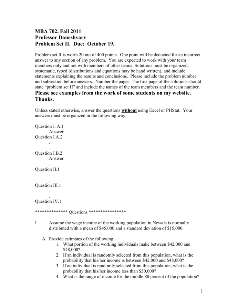
MBA 702, Fall 2011
Professor Daneshvary
Problem Set II. Due: October 19.
Problem set II is worth 20 out of 400 points. One point will be deducted for an incorrect
answer to any section of any problem. You are expected to work with your team
members only and not with members of other teams. Solutions must be organized,
systematic, typed (distributions and equations may be hand written), and include
statements explaining the results and conclusions. Please include the problem number
and subsection before answers. Number the pages. The first page of the solutions should
state “problem set II” and include the names of the team members and the team number.
Please see examples from the work of some students on my website.
Thanks.
Unless stated otherwise, answer the questions without using Excel or PHStat. Your
answers must be organized in the following way:
Question I. A.1
Answer
Question I.A.2
.
.
Question I.B.2
Answer
.
Question II.1
.
.
Question III.1
.
.
Question IV.1
.
************** Questions ****************
I.
Assume the wage income of the working population in Nevada is normally
distributed with a mean of $45,000 and a standard deviation of $15,000.
A. Provide estimates of the following:
1. What portion of the working individuals make between $42,000 and
$48,000?
2. If an individual is randomly selected from this population, what is the
probability that his/her income is between $42,000 and $48,000?
3. If an individual is randomly selected from this population, what is the
probability that his/her income less than $30,000?
4. What is the range of income for the middle 80 percent of the population?
1
5. From the actual data I found that about 20% of working people make
between $42,000 and $48,000. Explain the reason for the different result
obtained in part A.1.
B. Now we select a sample of 100 people from the population. Based on the sample:
1. What portion of the working individuals make between $42,000 and
$48,000?
2. What is the range of income for the middle 80 percent of the sample?
3. Explain why the answers to A.1 and B.1 differ.
II.
Now assume that we do not know the population’s average income but know its
(population’s) average dispersion (standard deviation) is $20,000.
1. What sample size is needed in order to estimate the true population mean
with 95% confidence that the sample result is correct to within a $2,000
margin of error.
A sample of 400 individuals is taken and the sample mean is calculated to be
$42,000. (We still know the population standard deviation).
2. Set up a 99% confidence interval estimate of the true population mean
income.
3. Explain why an individual with $70,000 income is not unusual.
4. Recalculate II.2, assuming that you do not have the population standard
deviation, but the sample standard deviation is $15,000.
III.
A corporation that hires an educated labor force is considering the possibility of a
branch in Nevada. To avoid extra expenses of relocating a trained labor force, the
corporation policy requires that it open branches in communities that have a
sufficiently educated local labor force. Suppose you are hired by the corporation
to do a study to determine if Nevada is a good location potential. You want to
estimate the average years of education. Based on national-level studies, the
standard deviation is 3.0 years.
1. The company requires the population to have a minimum of 14 years of
education. Set up the null and alternative hypotheses. Within the context
of this problem, explain the Type I and Type II errors and the risk and
consequences of committing them.
2. Now assume that you obtained a sample of 400 individuals. The sample
mean for the years of education is 13.7. Is there evidence (alpha 5
percent) that Nevada does not meet the requirement for branch location?
3. In fact, if the true population mean is 14 (the hypothesized value), what is
the probability of obtaining a sample mean that is 0.3 or more years (1413.7=.3) less than the population mean?
2
IV.
The sample of 811 working men and women in Nevada show the following
descriptive statistics about years of education and hours worked per week.
Mean
Std Dev.
No. of Obs.
Years of Education
Men
Women
Hours worked per Week
Men
Women
13.35
2.29
506
45
8.67
13.57
2.05
305
42
4.86
Without using PHStat, answer the following questions:
1. Using the 0.01 level of significance, is there evidence that average years of
education is different between men and women?
2. Using the 0.05 level of significance, is there evidence that the average
number of hours worked per week is different between men and women?
3. What assumption must be made in order to perform the test in (2)?
4. Using the 0.05 level of significance, is there evidence of a difference in
the variability of the hours worked per week between men and women?
5. Based on the result of (4), is it appropriate to use the test in (2)? Explain.
3