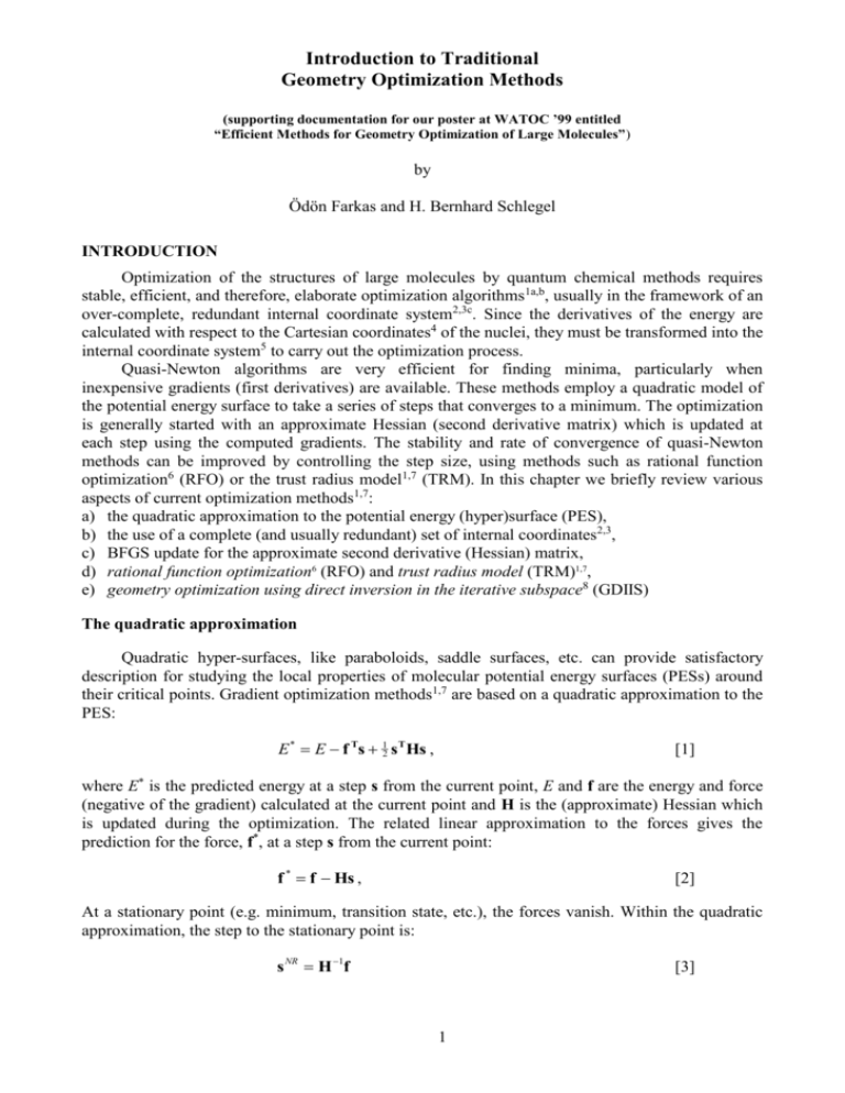
Introduction to Traditional
Geometry Optimization Methods
(supporting documentation for our poster at WATOC ’99 entitled
“Efficient Methods for Geometry Optimization of Large Molecules”)
by
Ödön Farkas and H. Bernhard Schlegel
INTRODUCTION
Optimization of the structures of large molecules by quantum chemical methods requires
stable, efficient, and therefore, elaborate optimization algorithms1a,b, usually in the framework of an
over-complete, redundant internal coordinate system2,3c. Since the derivatives of the energy are
calculated with respect to the Cartesian coordinates4 of the nuclei, they must be transformed into the
internal coordinate system5 to carry out the optimization process.
Quasi-Newton algorithms are very efficient for finding minima, particularly when
inexpensive gradients (first derivatives) are available. These methods employ a quadratic model of
the potential energy surface to take a series of steps that converges to a minimum. The optimization
is generally started with an approximate Hessian (second derivative matrix) which is updated at
each step using the computed gradients. The stability and rate of convergence of quasi-Newton
methods can be improved by controlling the step size, using methods such as rational function
optimization6 (RFO) or the trust radius model1,7 (TRM). In this chapter we briefly review various
aspects of current optimization methods1,7:
a) the quadratic approximation to the potential energy (hyper)surface (PES),
b) the use of a complete (and usually redundant) set of internal coordinates2,3,
c) BFGS update for the approximate second derivative (Hessian) matrix,
d) rational function optimization6 (RFO) and trust radius model (TRM)1,7,
e) geometry optimization using direct inversion in the iterative subspace8 (GDIIS)
The quadratic approximation
Quadratic hyper-surfaces, like paraboloids, saddle surfaces, etc. can provide satisfactory
description for studying the local properties of molecular potential energy surfaces (PESs) around
their critical points. Gradient optimization methods1,7 are based on a quadratic approximation to the
PES:
E *  E  f Ts  12 s T Hs ,
[1]
where E* is the predicted energy at a step s from the current point, E and f are the energy and force
(negative of the gradient) calculated at the current point and H is the (approximate) Hessian which
is updated during the optimization. The related linear approximation to the forces gives the
prediction for the force, f*, at a step s from the current point:
f *  f  Hs ,
[2]
At a stationary point (e.g. minimum, transition state, etc.), the forces vanish. Within the quadratic
approximation, the step to the stationary point is:
s NR  H 1f
[3]
1
Equation [3] is the definition of the well-known Newton-Raphson (NR) or quasi-Newton
optimization step, sNR, which is repeated until the optimization converges. If the quadratic
approximation described the PES accurately and the exact Hessian were used, then eq. [3] would
reach the stationary point in one step. However, the PES is not quadratic and the actual Hessian
provides a good approximation to the PES only in the vicinity of the current point, which may be
far from a stationary point (it may not even have the correct structure for the desired optimization zero negative eigenvalues for minimization, one negative eigenvalue for transition structure
searches). Furthermore, the calculation of the Hessian can be very expensive, specially for large
systems. Consequently, a quasi-Newton optimization usually starts with an approximate Hessian
matrix that has the required structure, and then improves the Hessian with an updating procedure
during the course of the optimization.
Regular coordinate transformations ( O(N3) )
The performance of the optimization process depends highly on the choice of the coordinate
system. In most cases the optimization is carried out in a complete internal coordinate system using
the derivatives computed with respect to Cartesian coordinates. The use of internal coordinates for
geometry optimization necessitates the transformation of the forces or gradients, calculated in
Cartesian coordinates, into internal coordinates and the back-transformation of the internal
coordinate optimization step into Cartesians. Usually both transformations are carried out with the
Wilson B-matrix9 used in vibrational spectroscopy. The connection between the Cartesian and
internal coordinate spaces is given by
dqint.  Bdq x ,
[4]
where dqint. and dqx. are the infinitesimal changes in the internal and Cartesian coordinates,
respectively, and B is the matrix of derivatives of the internal coordinates with respect to the
Cartesian coordinates. The corresponding connection between the internal forces, fint., and Cartesian
forces, fx, is
f x  B T f int . .
[5]
The forces are the negative of the potential energy gradients. Since the Wilson B-matrix is not
square, the transformation of the Cartesian force vector, fx, into the internal coordinate space is
usually written in terms of the inverse of the G matrix, where G  BB T (the atomic masses are
chosen to be unity):
fint  G 1Bf x ,
[6]
A generalized inverse should be used, since G is singular if the internal coordinate system contains
redundancy2,3c. The generalized inverse can be calculated via diagonalization, which requires a
number of O(N3) operations.
The forces in internal coordinates are used to update the Hessian and to predict the change in
geometry using either a Newton-Raphson or rational function optimization (RFO)6 step. The
transformation of the optimization step in internal coordinates (qint.) back to Cartesian coordinates
(qx.) is curvilinear, but can be carried out by iterating the following equation until the final
Cartesian coordinates yield the desired internal coordinates3a:
q x  B TG 1qint. .
[7]
In practice, the inverse of G is typically formed only once and is used to iterate eq. [7] until dqint.
and/or dqx. converges. This approach can be used for a small step, but the transformation of a large
2
step or the generation of a new structure may necessitate the recalculation of B, G and G 1 at each
iteration.
Hessian update
For minimizations within the quadratic model, the Hessian must be positive definite, for
which there are a number of suitable updating methods7. One of the most successful schemes is the
BFGS Hessian update10:
H k  H k 1  H kBFGS
 f f T H s sT H 
H kBFGS   T k k  k T1 k 1 k 1 k 1 
s k 1H k 1s k 1 
 s k 1f k
[8]
f k  f k  f k 1
However, the BFGS update converges to the actual Hessian only if accurate line searches are
used7d. The steps in typical molecular geometry optimizations usually do not meet this criterion
and, therefore, inaccuracies in the Hessian may lead to reduced efficiency near the end of an
optimization. A possible remedy for this behavior is to occasionally restart the update7.
Alternatively, the symmetric rank one (SR1) update (also known as the Murtagh-Sargent, update)11,
1
H k  H k 1  H SR
k
H
SR1
k
 f

 H k 1s k 1  f k  H k 1s k 1  ,
T
k
 f
[9]
 H k 1s k 1  s k 1
T
k
converges to the correct Hessian on a quadratic surface without exact line searches. However, this
update is unsuitable if the denominator becomes too small.
For transition state searches, the update should not force the Hessian to be positive definite.
The SR1 update is appropriate, as is the Powell-symmetric-Broyden12 (PSB) update:
H k  H k 1  H kPSB
H kPSB   f k  H k 1s k 1  s k 1
T
 f
k
s k 1sTk 1
s

2
T
k 1 k 1
s

 H k 1s k 1 sTk 1  s k 1  f k  H k 1s k 1 
sTk 1s k 1
[10]
T
Bofill developed an improved update13 by combining PSB with SR1 in a manner that avoids the
problem with the denominator of the latter:
1
H k  H k 1   Bofill H SR
 1   Bofill H kPowell
k
 Bofill 
f
f
 H k 1s k 1  s k 1
T
k
2
 H k 1s k 1   f k  H k 1s k 1 sTk 1s k 1
T
k

3
[11]
[12]
Trust radius model7 (TRM) and rational function optimization6 (RFO)
A simple quasi-Newton optimization based on a quadratic model with updated Hessians and
Newton-Raphson steps can readily encounter difficulties. Even when the Hessian has the right
structure (e.g. positive definite for minimizations), care must be taken not to step too far, since the
quadratic model is accurate for only a small region of the potential energy surface. Both RFO and
TRM can be regarded as methods for controlling the step size and have proven to be valuable
components of optimization algorithms. TRM and RFO based minimization algorithms can be
regarded as Newton-Raphson methods with a corrected Hessian:
s   H  S f
1
[13]
where  is a non-negative scalar, S is usually simply a constant scalar times the unit matrix, I, and
s is the resulting corrected step.
Trust radius model (TRM). The goal of TRM in minimization is to find the lowest energy point
within a suitable trust radius, in the framework of the quadratic approximation. This condition is
equivalent to finding a step, s, such that it is parallel to predicted force, f, points in the same
direction (  0) and has a length no greater than the trust radius, :
f   s 
[14]
s   f  Hs 
[15]
s  
[16]
and
Note that eq. [15] is equivalent to eq. [13] if S is replaced by the unit matrix. Equations [14-16]
have only one non-negative solution for  when the Hessian is positive definite ( is zero if the
length of the Newton-Raphson step is less than the trust radius). If the Hessian has one or more
negative eigenvalues, the only acceptable solution for minimization is always larger than the
negative of the lowest eigenvalue, lowest. Combining these conditions yields:
  Max 0, lowest 
[17]
The TRM method usually results in more efficient step size control than a simple scaling to the
Newton-Raphson step.
Rational function optimization (RFO). In the RFO approach for minimization, the quadratic model
is modified so that a suitably controlled step toward the minimum is obtained. By including a step
size dependent scaling denominator, the RFO method contains a self-consistent trust radius:
f Ts  12 s T Hs
,
E E
1  s TSs
[18]
*
where S is a symmetric, usually diagonal scaling matrix. The RFO approximation for the PES can
be expressed more compactly in terms of the augmented Hessian:
4
E*  E 
s
1
2
 H  f  s
1 T
0  1
 f
.
S 0 s
T
s 10 1 1

 
T
[19]
The expression of the force vector in terms of the RFO model is:
f  Hs  2 E *  E Ss
f 
1  s TSs
f  Hs 2f Ts  s T Hs


Ss
1  s TSs (1  s TSs )2
*
[20]
For the RFO step, sRFO, which satisfies the stationary condition, f* = 0, the predicted energy
lowering is E*-E = ½fTsRFO (i.e. same form as for the Newton-Raphson step in the quadratic
approximation). Thus the RFO step can be calculated by solving the implicit formula:

s RFO  H   f Ts RFO S

1
f   H  S f ,
1
[21]
where  = fTsRFO. In practice, S is chosen to be the identity (I), a scalar time the identity (I), or
some other diagonal matrix, yielding an RFO correction that is a simple diagonal shift of the
Hessian. Equation [21] can be expressed in the eigenvector space of the Hessian, where the H+S
matrix is diagonal and its inverse can be given explicitly. Some implementations split the
eigenvector space into subspaces for the “high” and “low” eigenvalues and solve eq. [21] for them
separately. This approach allows the extension of the RFO method for transition state optimizations
and is known as eigenvector following14 (EF) optimization.
Equation [21] is in implicit form; therefore, the solution can only be obtained by iterating
until  converges. For minimizations,  should obey condition [17] to ensure the positive
definiteness of H + S. Constraints on  for transition state optimizations are discussed
elsewhere.6b. Some important features of the RFO approach for minimization are:
a) smooth convergence to the quadratic approximation in the vicinity of critical points,
b) automatic scaling down of displacements corresponding to small eigenvalues of a positive
definite Hessian,
c) scaling up of displacement(s) corresponding to negative eigenvalues of the Hessian and
directing the step toward a minimum,
d) avoiding problems when the Hessian is nearly singular, such as in the vicinity of inflection
points.
5
Geometry optimization using direct inversion in the iterative subspace8 (GDIIS) method.
The quadratic potential energy surfaces (PESs) have some interesting features which are used
for multi-dimensional search (MDS) methods, like GDIIS. The linear search can use data (energy
and derivatives) computed only at two points but more efficiently than the quadratic approximation
(e.g. by fitting a quartic polynomial). The current MDS methods, like GDIIS, are based on the
quadratic approximation and using only the previous forces and geometry points with or without an
approximate Hessian. We assume in the following discussion that the forces are available for k
(k > 1) earlier points on a quadratic PES, described by eq. [1 and 2]. The k geometry points (qi,
i = 1..k) span a maximum k - 1 dimensional subspace, the iterative subspace. Any point of this
subspace (q*) can be produced using one of the geometrical points (e.g. q1) and a linear
combination of the available step vectors (sj = qj - q1, j = 2..k) connecting the chosen geometry
point to the other k - 1 points:
k
k
j 2
j 2


k
q*  q1    js j  q1    j q j  q1    i q i ,
[22]
i 1
where the i coefficients are defined as:
k
1  1    j
[23]
j 2
 j   j , j = 2.. k
and therefore
k

i
1
[24]
i1
The force (f*) at point q* can also be expressed using the same coefficients:
k
k
j 2
j 2


k
f  f1    j Hs j  f1    j f j  f1    i f i
*
[25]
i 1
Similar expressions can be constructed for any data if their changes have linear connection to the
changes in coordinates, like the first derivatives of a quadratic PES. The reversed statements of the
previous discussion are also valid:
a) When k points are given in a space, any linear combination of the related position vectors, if the
sum of the coefficients is 1 (condition [24]), will lead to a point which is in the subspace
spanned by the given points (eq. [22]).
b) Any data, if the data change has linear connection to the changes of the coordinates, can be
expressed as the same linear combination of the corresponding data at the given points. (See
eq. [25])
The goal of the GDIIS method is to find the coefficients which satisfy condition [24] and
minimizes the predicted data with a given measure, like the absolute value in the case of the forces.
The GDIIS based optimization methods in quantum chemistry use more efficient error vectors
instead of the gradients or forces to benefit from the information stored in the approximate Hessian.
The original GDIIS technique uses the Newton-Raphson (NR) steps (eq. [3]) as error vectors
calculated for the stored geometry points:
e i  s iNR  H 1f i
[26]
6
The appropriate linear combination of these error vectors leads to the prediction of the NR step
from the corresponding point:
k
e   iei
[27]
*
i 1
The task is to find proper ci coefficients which lead to the minimal length error vector, the residuum
vector, r, and hold condition [24]:
k
c e
r,
[28]
r is minimal and
[29]
i i
i 1
k
c
i
1
[30]
i1
The solution of this problem can be reached using the method of least squares by solving the
following system of linear equations:






 1  1
A
1  c1   0
   
     
    
1  c   0
k
   
0     1
[31]
where  is the Lagrangian multiplier and matrix A is the overlap matrix of the error vectors,
i, j
A  eie j .
The regular GDIIS algorithm begins with a Newton-Raphson step [2]. Subsequently the
method produces the DIIS coefficients solving the system of equations [31] using the set of
estimated error vectors calculated from the earlier (k) force vectors [26] and inverting the DIIS
matrix. Applying the given DIIS coefficients to the geometry vectors and error vectors, we get an
intermediate point (q*) and the residuum vector respectively. With the current definition of error
vectors the step by the residuum vector from the intermediate point gives the new geometry point
k


k
q k 1  q*  r   ci q i  e i   ci q iNR .
i=1
[32]
i=1
The new geometry point can be regarded as the same linear combination of the predicted
geometry points ( q iNR  q i  s iNR ) produced by Newton-Raphson steps from the corresponding
points.
7
References
1
(a) H. B. Schlegel “Geometry optimization on potential energy surfaces” in Modern Electronic
Structure Theory D. R.. Yarkony, ed., (World Scientific Publishing, 459-500, 1995)
(b) H. B. Schlegel “Geometry optimization” in Encyclopedia of Computational Chemistry
(Wiley, New York, 1998)
2
C. Peng, P. Y. Ayala, H. B. Schlegel and M. J. Frisch, J. Comp. Chem. 17, 49-56 (1996)
3
(a) P. Pulay, G. Fogarasi, F. Pang and J. E. Boggs, J. Am. Chem. Soc. 101, 2550 (1979)
(b) G. Fogarasi, X. Zhou, P. W. Taylor and P. Pulay, J. Am. Chem. Soc. 114, 8191 (1992)
(c) P. Pulay and G. Fogarasi, J. Chem. Phys. 96, 4 (1992)
4
P. Pulay, in Ab initio Methods in Quantum Chemistry. Part II, Adv. Chem. Phys. 69, (1986)
5
P. Pulay, Mol. Phys. 17, 197 (1969)
6
(a) A. Banerjee, N. Adams, J. Simons and R. Shepard, J. Phys. Chem. 89, 52 (1985)
(b) J. Simons and J. Nichols, Int. J. Quantum Chem., Quantum Chem. Symp. 24, 263 (1990)
7
(a)
(b)
(c)
(d)
8
(a) P. Pulay, Chem Phys. Letters 73, 393 (1980)
(b) P. Pulay, J. Comp. Chem. 3, 556 (1982)
(c) P. Császár and P. Pulay, J. Mol. Struct. (THEOCHEM) 114, 31 (1984)
R. Fletcher Practical Methods of Optimization (Wiley, Chichester, 1981)
W. Murray and M. H. Wright Practical Optimization (Academic Press, New York, 1981)
M. J. D. Powell, ed. Non-linear Optimization, 1981 (Academic Press, New York, 1982)
J. E. Dennis and R. B. Schnabel Numerical Methods for Unconstrained Optimization and
Non-Linear Equations (Prentice Hall, New Jersey, 1983)
(e) L. E. Scales Introduction to Non-linear Optimization (Macmillam, Basingstoke, 1985)
9
E. B. Wilson, J. C. Decius and P. C. Cross, Molecular vibrations, McGraw-Hill, New-York,
(1955)
10 (a)
(b)
(c)
(d)
C. G. Broyden, J. Inst. Math. Appl. 6, 76 (1970)
R. Fletcher, Comput. J. 13, 317 (1970)
D. Goldfarb, Math. Comput. 24, 23 (1970)
D. F. Shanno, Math. Comput. 24, 647 (1970)
11
B. Murtagh and R. W. H. Sargent, Comput J. 13, 185 (1972)
12 (a) M. J. D. Powell, in Nonlinear Programing, eds. J. B. Rosen, O. L. Mangasarian and K.
Ritter (Academic, New York, 1970)
(b) M. J. D. Powell, Math. Prog. 1, 26 (1971)
13
J. M. Bofill, J. Comp. Chem. 15, 1 (1994)
14
J. Baker, J. Comp. Chem. 7, 385 (1986)
15
J. Baker, J. Comp. Chem. 14, 1085 (1993)
16
C. van Alsenoy, C.-H. Yu, A. Peeters, J. M. L. Martin and L. Schäfer, J. Phys. Chem. 102,
2246 (1998)