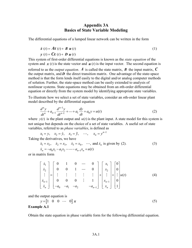
Appendix 3A
Basics of State Variable Modeling
The differential equations of a lumped linear network can be written in the form
(1)
x (t )  Ax (t )  B u (t )
y (t )  Cx (t )  D u (t )
This system of first-order differential equations is known as the state equation of the
system and x (t ) is the state vector and u (t ) is the input vector. The second equation is
referred to as the output equation. A is called the state matrix, B the input matrix, C
the output matrix, and D the direct transition matrix. One advantage of the state-space
method is that the form lends itself easily to the digital and/or analog computer methods
of solution. Further, the state-space method can be easily extended to analysis of
nonlinear systems. State equations may be obtained from an nth-order differential
equation or directly from the system model by identifying appropriate state variables.
To illustrate how we select a set of state variables, consider an nth-order linear plant
model described by the differential equation
dny
d n1 y
dy
(2)

a
  a1  a0 y  u (t )
n1
n
n1
dt
dt
dt
where y (t ) is the plant output and u (t ) is the plant input. A state model for this system is
not unique but depends on the choice of a set of state variables. A useful set of state
variables, referred to as phase variables, is defined as
x1  y, x2  y, x3  y,
, xn  y n1
Taking the derivatives, we have
(3)
x1  x2 , x2  x3 , x3  x4 ,
, and xn is given by (2).
xn  a0 x1  a1x2   an1xn  u (t )
or in matrix form
 x1   0
 x   0
 2  



 
 xn 1   0
 xn    a0
1
0
0
1
0
0
 a1  a2
0   x1  0 
0   x2  0 
 

    u (t )
 
  
1   xn 1  0 
 an 1   xn  1 
and the output equation is
y  1 0 0
0 x
Example A.1
(4)
(5)
Obtain the state equation in phase variable form for the following differential equation.
3A.1
d3y
d2y
dy

4
 6  8 y  10u(t )
3
2
dt
dt
dt
The differential equation is third order, thus there are three state variables as follows
x1  y, x2  y, x3  y
and the derivatives are
x1  x2 , x2  x3 , and x3  4 x1  3x2  2 x3  5u(t )
Or in matrix form
2
 x1   0 1 0   x1  0 
 x    0 0 1   x   0  5u (t )
 2 
 2  
 x3   4 3 2   x3  1 
 x1 
y  1 0 0  x2 
 x3 
The M-file ode2phv.m is developed which converts an nth-order ordinary differential
equation to the state-space phase variable form. [A, B, C] = ode2phv(ai, k) returns the
matrices A, B, C, where ai is a row vector containing coefficients of the equation in
descending order and k is the coefficient of the right-hand side.
ai = [2 4 6 8];
k = 10;
[A, B, C] = ode2phv(ai, k)
produces the following phase variable state representation
A=
B =
C =
0 1 0
0
1 0 0
0 0 1
0
-4 -3 -2
5
Equations of Electrical Networks
The state variables are directly related to the energy-storage elements of a system. It
would seem, therefore, that the number of independent initial conditions is equal to the
number of energy-storing elements. This is true provided that there is no loop containing
only capacitors and voltage sources and there is no cut set containing only inductive and
current sources. In general, if there are nc loops of all capacitors and voltage sources, and
nL cut sets of all inductors and current sources, the number of state variables is
n  eL  eC  nC  nL
(6)
where
eL = number of inductors
eC = number of capacitors
3A.2
nC = number of all capacitive and voltage source loops
nL = number of all inductive and current source cut sets
Example A.2
Write the state equation for the network shown in Figure A.1.
2H
vc 2
4  vc1
iL
vi

-
0.25 F
0.5 F
1
is
0
Figure A.1 Circuit of Example 2
Define the state variables as current through the inductor and voltage across the
capacitors. Write two node equations containing capacitors and a loop equation
containing the inductor. The state variables are vc1, vc2 , and iL .
Node equations are
dv
v v
0.25 c1  iL  c1 i  0

dt
4
dv
v
0.5 c 2  iL  c 2  is  0

dt
1
and the loop equation is
di
2 L  vc 2  vc1  0

dt
or
0
4  vc1  1
 vc1   1
v    0
2
2  vc 2   0
 c2  
 iL  0.5 0.5 0   iL  0
vc  vc1  4iL  vi
vc 2  2iL  2vc 2  2is
iL  0.5vc1  0.5vc 2
0
v 
2  i 
i
0   s 
Simulation Diagram
Equation (3) indicates that state variables are determined by integrating the
corresponding state equation. A diagram known as the simulation diagram can be
constructed to model the given differential equations. The basic element of the simulation
diagram is the integrator. The first equation in (3) is
x1  x2
Integrating, we have
x1   x2 dx
3A.3
The above integral is represented by the time-domain diagram shown in Figure 2 (a)
similar to the block diagram or the time-domain diagram shown in Figure 2 (b) similar to
the signal flow graph.
x2 (t )
s 1
x1 (t )
1
s
x2 (t )
x1 (t )
(b)
(a)
Figure A.2 Simulation diagram for integrator
It is important to know that although the symbol 1/ s is used for integration, the
simulation diagram is a time domain representation. The number of integrators is equal to
the number of state variables. For example, for the state equation in Example 1 we have
three integrators in cascade, the three state variables are assigned to the output of each
integrator as shown in Figure 3. The last equation in (3) is represented via a summing
point and feedback paths. Completing the output equation, the simulation diagram known
as phase-variable control canonical form is obtained.
5u (t )
x3
- -
-
1
s
2
x3
1
s
x2
1
s
x1
y
5u (t )
1
1
x3
s 1
s 1
s 1 1
x1
x2
-2 x3
-3
OR
3
-4
4
(a)
(b)
Figure A.3 Simulation diagram for Example 1
Transfer Function to State-Space Conversion
Direct Decomposition
Consider the transfer function of a third-order system
b s 2  b s  b0
Y ( s)
(7)
 3 2 2 1
U ( s) s  a2 s  a1s  a0
where the numerator degree is lower than that of the denominator. The above transfer
function is decomposed into two blocks as shown in Figure 4.
U (s)
1
3
2
s  a2 s  a1s  a0
W (s)
b2 s 2  b1s  b0
Y ( s)
Figure A.4 Transfer function (7) arranged in cascade form
Denoting the output of the first block as W ( s) , we have
U ( s)
and
W ( s)  3
Y (s)  b2 s2W (s)  b1sW (s)  b0W (s)
2
s  a2 s  a1s  a0
or
3A.4
y
s3W (s)  a2 s 2W (s)  a1sW (s)  a0W (s)  U (s)
This results in the following time-domain equation
w  a2 w  a1w  a0 w  u (t ) and
y(t )  b2 w  b1w  b0 w
From the above expression we see that w has to go through three integrators to get w as
shown in Figure 5. Completing the above equations results in the phase-variable control
canonical simulation diagram.
b2
b1
u (t )
1 w
x3
s
a2
w
- -
-
1 w
x2
s
1 w
x1
s
+ +
b0
+
y
a1
a0
Figure A.5 Phase variable control canonical simulation diagram.
The above simulation in block diagram form is suitable for SIMULINK diagram
construction. You may find it easier to construct the simulation diagram similar to the
signal flow graph as shown in Figure 6.
b2
b1
u (t )
1
w
s 1 w b0
s 1 w
s 1 w
x2
a2 x3
x1
a1
a0
1
y
Figure A.6 Phase variable control canonical simulation diagram.
In order to write the state equation, the state variables x1 (t ) , x2 (t ) , and x3 (t ) are assigned
to the output of each integrator from the right to the left. Next an equation is written for
the input of each integrator. The results are
x1  x2
x2  x3
x3  a0 x1  a1x2  a0 x1  u (t )
and the output equation is
y  b0 x1  b1x2  b3 x3
or in matrix form
3A.5
 x1   0
x    0
 2 
 x3   a0
0   x1  0
1   x2   0 u (t )
a2   x3  1 
1
0
a1
(8)
 x1 
y  1 0 0  x2 
 x3 
It is important to note that the Mason’s gain formula can be applied to the simulation
diagram in Figure 6 to obtain the original transfer function. Indeed  of Mason’s gain
formula is the characteristic equation. Also, the determinant of sI  A matrix in (8),
results in the characteristics equation. Keep in mind that there is not a unique state space
representation for a given transfer function.
The Control System Toolbox contains a set of functions for model conversion.
[A, B, C, D] = tf2ss(num, den) converts the system in transfer function from to statespace phase variable control canonical form.
Example A.3
For the following transfer function
Y ( s)
s 2  7s  2
G( s) 
 3
U ( s) s  9s 2  26s  24
(a) Draw the simulation diagram and find the state-space representation of the above
transfer function.
(b) Use MATLAB Control System Toolbox [A, B, C, D] = tf2ss(num, den) to find the
state model.
(a) Draw the transfer function block diagram in cascade form
U ( s)
W (s) 2
1
s  7s  2
3
2
s  9 s  26s  24
From this we have
s3W ( s)  9s 2W ( s)  26sW ( s)  24W ( s)  U ( s )
or in time-domain
&
Y (s)
Y ( s)  s 2W ( s)  7 sW ( s)  2W ( s)
w  9w  26w  24w  u & y  w  7 w  2w
The above time-domain equations yield the following simulation diagram
3A.6
1
7
1
u (t )
w
s 1 w 2
s 1 w
s 1 w
x2
x1
9 x3
26
1
y
24
To obtain the state equation, the state variables x1 (t ) , x2 (t ) , and x3 (t ) are assigned to the
output of each integrator from the right to the left. Next an equation is written for the
input of each integrator. The results are
x1  x2
x2  x3
x3  24 x1  26 x2  9 x1  u (t )
and the output equation is
y  2 x1  7 x2  x3
or in matrix form
1
0   x1  0
 x1   0
x    0
0
1   x2   0 u (t )
 2 
 x3   24 26 9  x3  1 
 x1 
y   2 7 1  x2 
 x3 
(b) We write the following statements
num = [1 7 2]; den = [1 9 26
[A, B, C, D] = tf2ss(num, den)
24];
The result is
A=
B=
-9
1
0
-26
0
1
-24
0
0
C=
1
0
0
D=
1
7
2
0
Note that MATLAB assigns x1 to the output of the first integrator, and x2 , and x3 to the
output of the second and third integrators.
3A.7
State-Space to Transfer Function Conversion
Consider the state and output equations
x (t )  Ax (t )  B u (t )
y  Cx (t )  D u (t )
Taking the Laplace transform
sX ( s )  AX ( s)  BU ( s)

[sI  A] X ( s)  BU ( s)
Y ( s )  CX ( s )  DU ( s)
Substituting for X ( s) in the second equation above, we get
Y ( s )  C[ SI  A]1 BU ( s )  DU ( s)
or
Y ( s)
 C[ SI  A]1 B  D
U ( s)
In MATLAB [num, den] = ss2tf(A, B, C, D, i) converts the state equation to a transfer
function for the ith input.
Example A.4
A system is described by the following state-space equations
 x1   0 1   x1  0
 x   6 5  x   1 u (t )
 2  
 2 
x 
y  [8 1]  1 
 x2 
Obtain the system transfer function using the formula in (3.18)
 s 1 
[ SI  A]  

 6 s  5
 s  5 1
 6
s 

1
 ( s)  [ SI  A]  2
s  5s  6
 s  5 1  0 
1
[8 1]  
 6



s  1 
s  8  s
G ( s )  C[ SI  A]1 B  [8 1]  2
 2
s  5s  6
s  5s  6 s 2  5s  6
Therefore
s 8
G( s)  2
s  5s  6
In MATLAB [num, den] = ss2tf(A, B, C, D, i) converts the state equation to a transfer
function for the ith input.
3A.8
Example A.5
A system is described by the following state-space equations
 x1   0 1 0   x1  10
 x    0 0 1   x    0  u (t )
 2 
 2  
 x3   1 2 3  x3   0 
(8)
 x1 
y  1 0 0  x2 
 x3 
Y ( s)
. The following statements:
U ( s)
A = [0 1 0; 0 0 1; -1 -2 -3]; B = [10; 0; 0];
C = [1 0 0]; D = [0];
[num, den] = ss2tf(A, B, C, D, 1)
G = tf(num, den)
results in
num =
0.0000 10.0000 30.0000 20.0000
den =
1.0000 3.0000 2.0000 1.0000
Transfer function:
10 s^2 + 30 s + 20
--------------------s^3 + 3 s^2 + 2 s + 1
Find the transfer function, G ( s) 
Also, [z, p] = ss2tf(A, B, C, D, 1) converts the state equation to transfer function in
factored form.
MALAB Control System Toolbox contains many functions for model creation and
inversion, data extraction, and system interconnections. A few of these functions for
continuous-time control systems are listed below. For a complete list of all functions type
help/control/control at MATLAB prompt.
tf
zpk
ss
tfdata
zpkdata
ssdata
append
parallel
series
feedback
connect
blkbuild
Create transfer function models.
Create zero/pole/gain models.
Create state-space models.
Extract numerator(s) and denominator(s).
Extract zero/pole/gain data.
Extract state-space matrices.
Group LTI systems by appending inputs and outputs.
Generalized parallel connection (see also overloaded +).
Generalized series connection (see also overloaded *).
Feedback connection of two systems.
Derive state-space model from block diagram description.
Builds a model from a block diagram.
3A.9
The Control System Toolbox supports four commonly used representations of linear
time-invariant (LTI) systems: tf, zpk, and ss objects. To create an LTI model or object,
use the corresponding constructor tf, zpk, or ss. For example,
sys = tf(1,[1 0]) .
creates the transfer function H(s) = 1/s. The result sys is a tf object containing the
numerator and denominator data. You can then manipulate the entire model as the single
MATLAB variable sys. For more details and examples on how to specify the various
types of LTI models, type ltimodels followed by tf, zpk, or ss.
The functions tfdata, zpkdata, and ssdata are provided for extracting the parameters of
the tf, zpk and ss objects. For example the command [num, den] = tfdata(T, 'v') returns
the numerator and denominator of the tf object. The argument ‘v’ returns the numerator
and denominator as row vectors rather than cell arrays. The Control System Toolbox
contains seven more functions, which are useful for creating a single model out of its
components.
Example A.6
Use feedback function to obtain the closed-loop transfer function and the tf2ss function
to obtain the closed-loop state-space model
R( s)

5( s  1.4)
s7
1
s ( s  1)( s  4)
G p ( s)
Gc ( s )
C ( s)
H ( s)
10
The following commands
Gc = tf(5*[1 1.4], [1 7])
Gp = tf([1], [1 5 4 0]);
H = 10;
G = series(Gc, Gp)
T = feedback(G, H)
[num, den] = tfdata(T, 'v');
[A, B, C, D]=tf2ss(num, den)
% transfer function Gc
% transfer function Gp
% connects Gc & Gp in cascade
% obtains the closed loop transfer function
% returns num & den as row arrays
% returns the A,B, C, D matrices
% of the state space model
result in
Transfer function:
5s+7
--------------------------------s^4 + 12 s^3 + 39 s^2 + 78 s + 70
3A.10
A=
B=
-12
1
0
0
-39
0
1
0
-78
0
0
1
-70
0
0
0
C=
1
0
0
0
D=
[0 0 5 7]
0
For analytical solution of state equation refer to the lecture notes on Chapter 3.
3A.11