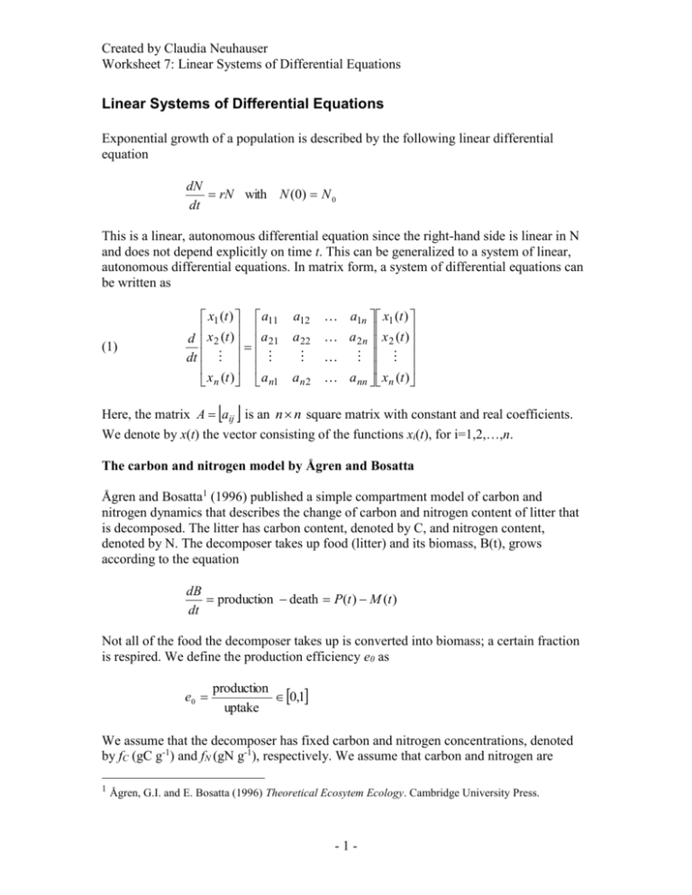
Created by Claudia Neuhauser
Worksheet 7: Linear Systems of Differential Equations
Linear Systems of Differential Equations
Exponential growth of a population is described by the following linear differential
equation
dN
 rN with N (0)  N 0
dt
This is a linear, autonomous differential equation since the right-hand side is linear in N
and does not depend explicitly on time t. This can be generalized to a system of linear,
autonomous differential equations. In matrix form, a system of differential equations can
be written as
(1)
 x1 (t )   a11

 
d  x 2 (t ) a 21

dt     

 
 x n (t )  a n1
a12
a 22

an2
 a1n   x1 (t ) 
 a 2n   x 2 (t ) 
    


 a nn   x n (t )
 
Here, the matrix A  aij is an n  n square matrix with constant and real coefficients.
We denote by x(t) the vector consisting of the functions xi(t), for i=1,2,…,n.
The carbon and nitrogen model by Ågren and Bosatta
Ågren and Bosatta1 (1996) published a simple compartment model of carbon and
nitrogen dynamics that describes the change of carbon and nitrogen content of litter that
is decomposed. The litter has carbon content, denoted by C, and nitrogen content,
denoted by N. The decomposer takes up food (litter) and its biomass, B(t), grows
according to the equation
dB
 production  death  P(t )  M (t )
dt
Not all of the food the decomposer takes up is converted into biomass; a certain fraction
is respired. We define the production efficiency e0 as
e0 
production
 0,1
uptake
We assume that the decomposer has fixed carbon and nitrogen concentrations, denoted
by fC (gC g-1) and fN (gN g-1), respectively. We assume that carbon and nitrogen are
1
Ågren, G.I. and E. Bosatta (1996) Theoretical Ecosytem Ecology. Cambridge University Press.
-1-
Worksheet 7: Linear Systems of Differential Equations
incorporated into biomass at rates f C P and f N P , respectively. If we denote the rate of
respiration by R, then carbon uptake is of the form [uptake]=[respiration]+[production]
(see Figure 1),
fC P
 R  fC P
e0
respiration
litter
decomposer
uptake
production
C
B
death
mineralization/
immobilization
decomposer
litter
uptake
production
N
B
death
Figure 1: Diagram of the carbon and nitrogen processes.
We assume that nitrogen uptake follows carbon uptake passively, that is, it is equal to the
carbon uptake rate times the nitrogen to carbon ratio (N:C) of the substrate.
Nitrogen uptake 
fC P N
e0 C
The difference between nitrogen uptake and production can be positive or negative. If it
is positive, decomposers release nitrogen (mineralization); if it is negative, decomposers
need to import nitrogen from the surroundings (immobilization).
To complete the dynamics, we need to include death of the decomposer. We
assume that both carbon and nitrogen of the decomposer are lost to the litter pool at rates
f C M and f N M , respectively.
This yields the following set of equations for the carbon and nitrogen dynamics of
the litter
-2-
Worksheet 7: Linear Systems of Differential Equations
f P
dC
  C  fC M
dt
e0
f PN
dN
 C
 fN M
dt
e0 C
We make the following assumptions: (1) mortality rate is equal to production rate, that is,
M  P , and (2) production rate is proportional to the carbon content of the litter, that is,
P  uC , where u is the constant of proportionality. Then,
(2)
If we define  
(3)
1  e0
dC

f C uC
dt
e0
f u
dN
  C N  f N uC
dt
e0
fCu
,   f N u, and   1  e0 , then this can be written
e0
dC
  C
dt
dN
 N   C
dt
Equation (3) is a linear system with matrix
(4)
 
A
 
0 
  
Approximating the Solution of a Differential Equation—Euler Method
Numerical analysis is a field in mathematics that is concerned with developing
approximate numerical methods and assessing their accuracy, for instance for solving
differential equations. We will discuss the simplest method, the Euler method, explain the
basic idea behind this numerical method, and how to implement it on a spreadsheet.
The Euler method is based on the definition of a derivative. Recall that the
derivative of a function f(x) at x is defined as
-3-
Worksheet 7: Linear Systems of Differential Equations
df
f ( x  x)  f ( x)
 lim
dx x0
x
provided that the limit exists. This can be used to approximate solutions of differential
equations numerically. Namely, to solve
dy
 g ( y ) with
dx
we approximate
y  y0 when x  x0
dy
y ( x  x)  y ( x)
by the difference quotient
. This yields
dx
x
y ( x  x)  y ( x) 
dy
x  y ( x)  g ( y )x
dx
This can be used iteratively starting with the initial condition.
To apply this to the system of differential equations that describes the carbon and
nitrogen dynamics, we find the iterative equations
(5)
C (t  t )  C (t )   C (t )t
N (t  t )  N (t )  N (t )t  C (t )t
This can be coded up in a spreadsheet. The accuracy of the approximation is determined
by the time step t . In theory, smaller time steps yield more accurate solutions. In
practice, however, if time steps are too small, numerical errors accumulate due to
rounding errors that are inevitable when using a computer.
Solving Differential Equations
A linear differential equation
dx
 rx with x(0)  x0
dt
has the solution
x(t )  x0e rt
The solution is thus given by an exponential function A system of linear, autonomous
differential equations
-4-
Worksheet 7: Linear Systems of Differential Equations
(6)
 x1 (t )   a11

 
d  x 2 (t ) a 21

dt     

 
 x n (t )  a n1
a12
a 22

an2
 a1n   x1 (t ) 
 a 2n   x 2 (t ) 
    


 a nn   x n (t )
 
where the matrix A  aij is an n  n square matrix with constant and real coefficients,
can be solved exactly and the solutions are also exponential functions. We denote by x(t)
the vector consisting of the functions xi(t), for i=1,2,…,n. Solutions to systems of linear,
autonomous differential equations are given by the exponential function of the form
x(t )  e t w
where λ is a constant and w is a constant vector. How do we need to choose λ and w so
dx
 Ax ? Let’s compute the left-hand side and the
that this is indeed a solution, that is,
dt
right-hand side of this equation:
dx
 e t w and Ax  e t Aw
dt
After equating the two expressions and canceling e t on both sides, we find
Aw  w
This implies that the function x(t )  e t w is a solution if λ is an eigenvalue
corresponding to the eigenvector w of the matrix A. We will explain below how to
compute eigenvalues and eigenvectors for a given square matrix A.
To find the general solution of a system of differential equations, note that if y(t)
and z(t) are both specific solutions, then their sum is also a solution. This follows from
the fact that the system of differential equations is linear:
d
 y(t )  z (t )   dy  dz  Ay  Az  A y(t )  z (t )
dt
dt dt
This is called the superposition principle.
We restrict ourselves to the case when A has eigenvalues λi that are all distinct
and real with corresponding eigenvectors wi. In this case, the general solution is of the
form
n
(7)
x(t )   ci e it wi
i 1
-5-
Worksheet 7: Linear Systems of Differential Equations
where the ci’s are determined from the initial condition.
Eigenvalues and Eigenvectors
Definition: Assume that A is a square matrix. A nonzero vector w that satisfies the
equation
(8)
Aw  w
is a (right) eigenvector of the matrix A and the number λ is the corresponding eigenvalue.
Note that we assume that the eigenvector is different from the zero vector. An eigenvalue
though can be 0, it can even be a complex number. To find eigenvectors and eigenvalues,
we need to solve the equation
Aw  w
We can rewrite this as
Aw  w  0
( A  I ) w  0
In order to obtain a nontrivial solution (i.e., w  0 ), the matrix A  I must be singular,
that is,
det( A  I )  0
Solving this equation will yield values for λ. For each value of λ, we can then find an
eigenvector w using Equation (8).
We assume now that all eigenvalues of the matrix A are distinct and real. In this
case, all the eigenvectors can be computed by solving Aw  w for each eigenvalue; the
eigenvectors are then real.
Task 1:
Show that the eigenvalues of A are
1  
and
2  
with corresponding
eigenvectors
 1   
w1  

  
and
0 
w2   
1
Use (7) to show that the solution with initial conditions C(0) and N(0) is given by
-6-
Worksheet 7: Linear Systems of Differential Equations
C (t )  C (0)e t
N (t )  N (0)e t 

C (0) t
e
 e t
 (1   )
-7-

Worksheet 7: Linear Systems of Differential Equations
Computer Lab (due __________________)
We will numerically solve the compartment model of carbon and nitrogen dynamics by
Ågren and Bosatta (1996) using Euler’s method. We will use the parameters
e0  0.2, f C  0.5, f N  0.05, u  0.0004 d 1 , and set the N:C ratio of the substrate at time
0 equal to 0.01.
Step 1
Open the EXCEL spreadsheet (Tab: “Steps 1-3, Step 5”): The following cells are relevant
for Step 1:
A
B
C
D
E
F
G
H
1 Carbon and Nitrogen Dynamics
2
3 e_0
f_C
f_N
u
N:C (time 0) C_0
N_0
Delta t
4
0.2
0.5
0.05
0.0004
0.01
20
0.2
0.5
5
6
7 Time
C(t)
N(t)
N/N_0
C/C_0
N/C
8
0
20
0.2
1
1
0.01
Cells A4 to F4 are entered as values. Cell G4 contains “=$E$4*$F$4” and cell H4 is a
value. Enter “0” into cell A8, “=$F$4” into cell B8, “=$G$4” into cell C8, “=C8/$G$4”
into cell D8, “=B8/$F$4” into E8, and “=C8/B8” into F8.
Step 2
We will use the Euler method to solve the system of differential equations
1  e0
dC

f C uC
dt
e0
f u
dN
  C N  f N uC
dt
e0
numerically. The iterative equations are given by
C (t  t )  C (t ) 
1  e0
f C uC (t )t
e0
N (t  t )  N (t ) 
fC u
N (t )t  f N uC (t )t
e0
-8-
Worksheet 7: Linear Systems of Differential Equations
The iterative equations are entered into your spreadsheet for the first time step. The
relevant cells in your spreadsheet look as follows:
A
B
C
D
E
F
G
H
1 Carbon and Nitrogen Dynamics
2
3 e_0
f_C
f_N
u
N:C (time 0) C_0
N_0
Delta t
4
0.2
0.5
0.05
0.0004
0.01
20
0.2
0.5
5
6
7 Time
C(t)
N(t)
N/N_0
C/C_0
N/C
8
0
20
0.2
1
1
0.01
9
0.5
19.992
0.2001
1.0005
0.9996 0.010009
A9: =A8+$H$4
B9: =B8-(1-$A$4)*$B$4*$D$4*B8*$H$4/$A$4
C9: =C8-$B$4*$D$4*C8*$H$4/$A$4+$C$4*$D$4*$H$4*B8
D9: =C9/$G$4
E9: =B9/$F$4
F9: =C9/B9
Drag Row 9 down to about 3000 time steps and graph N/N0, C/C0, and N/C as functions
of time in one coordinate system where N0 and C0 are the nitrogen and carbon litter
contents at time 0.
Step 3
Solve the system of differential equations numerically using the Euler method for the
following set of N:C ratios: (a) N:C=0.01, (b) N:C=0.1, and (c) N:C=0.3. Graph N/N0,
C/C0, and N/C as functions of time in one coordinate system for each of the three cases.
Homework (due ____________________)
Step 4
Explain the following statements using your graphs from Step 3: (A) When N:C ratio of
the food is less than that of the microbes, the microbes take up nitrogen from the
surrounding soil. (B) When the N:C ratio of the litter is equal to that of the microbes, the
decline of N/N0 and C/C0 are identical—the food is perfectly balanced. When N:C ratio
of the food is higher than that of the microbes, the microbes need not take up any
nitrogen from the surrounding environment.
-9-
Worksheet 7: Linear Systems of Differential Equations
Step 5
Go back to the Tab “Steps 1-3, Step 5”). Columns I-N are now used. Enter the exact
solution into the spreadsheet and plot the remaining fractions of carbon and nitrogen (i.e.,
C(t)/C(0) and N(t)/N(0)) together with the N:C ratio of the litter as functions of time in
one coordinate system. Evaluate how accurate the approximation is as a function of t .
Step 6
The paper by Olson (Ecology 44(2), 1963, 322-331) describes a decay model with input
(Equation 2)
(8)
dX
 L  kX
dt
Where X (t ) denotes the amount of organic carbon in dead organic matter per square
meter of ground surface (measured in grams). Equation (6) in Olson’s paper is identical
dC
  C ).
to the carbon decay model in this module (Equation 3,
dt
(a) Set L  0 in Equation (8) and solve the resulting equation with the initial condition
X (0)  X 0 (use paper and pencil). What is the fraction X (t ) / X (0) that remains at time t?
1
to solve Equation (8)
365
numerically in EXCEL for two cases: (i) continuous litter fall (case 1) and (ii) discrete
annual litter fall (case 2). In each case assume that the total amount of litter that is added
per year per square meter of ground surface is 200 grams. Assume that k=1 and X(0)=0,
and run each model long enough so that the model has time to stabilize (i.e., the longterm pattern becomes clear). In your write-up produce a graph of X (t ) for each case.
(b) Use the Euler approximation with time step t 
(c) In Olson (1963) on page 325, the following statement is made:
Because kX is higher in the first half of each annual cycle than in the second half,
the steady state of the smooth curve lies a little below the half-way level between
peaks and troughs for the discontinuous case.
Confirm this statement with the solutions you found.
- 10 -