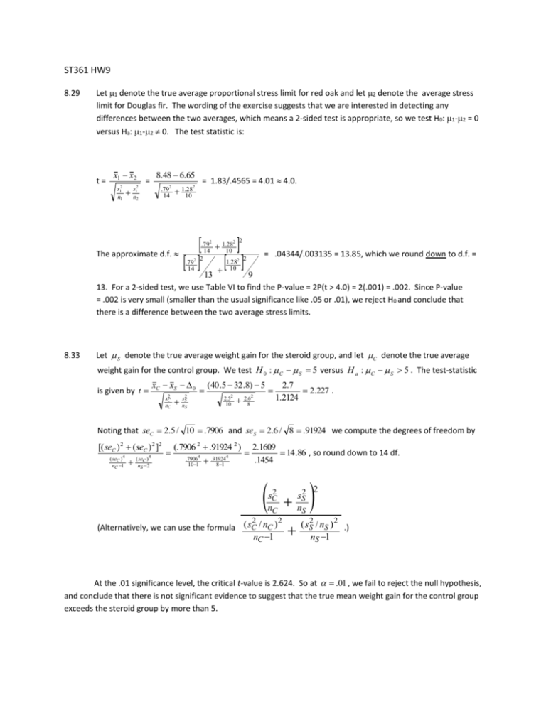
ST361 HW9
8.29
Let 1 denote the true average proportional stress limit for red oak and let 2 denote the average stress
limit for Douglas fir. The wording of the exercise suggests that we are interested in detecting any
differences between the two averages, which means a 2-sided test is appropriate, so we test H0: 1-2 = 0
versus Ha: 1-2  0. The test statistic is:
t=
x1  x2
s12

n1
s12
=
n2
8.48  6.65
.792
14
= 1.83/.4565 = 4.01  4.0.
28
 1.10
2

The approximate d.f. 
 
.792
14
.792
14
2
2
28
 1.10

2
 

1.282
10
= .04344/.003135 = 13.85, which we round down to d.f. =
2
13
9
13. For a 2-sided test, we use Table VI to find the P-value = 2P(t > 4.0) = 2(.001) = .002. Since P-value
= .002 is very small (smaller than the usual significance like .05 or .01), we reject H 0 and conclude that
there is a difference between the two average stress limits.
8.33
Let  S denote the true average weight gain for the steroid group, and let  C denote the true average
weight gain for the control group. We test H 0 :  C   S  5 versus H a :  C   S  5 . The test-statistic
is given by t 
xC  xS   0
sC2
nC

sS2
nS

(40 .5  32 .8)  5
2
2.5
10

2.6
8

2
2.7
 2.227 .
1.2124
Noting that seC  2.5 / 10  .7906 and seS  2.6 / 8  .91924 we compute the degrees of freedom by
[( seC ) 2  (seC ) 2 ]2
4
( seC )
nC 1

4
( seC )
nS 2

(.7906 2  .91924 2 ) 2.1609

 14 .86 , so round down to 14 df.
.79064
.919244
.1454
101  81

sC2
nC
2
2
(Alternatively, we can use the formula ( sC / nC )
nC 1


sS2
nS

2
( sS2 / nS ) 2 .)
nS 1
At the .01 significance level, the critical t-value is 2.624. So at   .01 , we fail to reject the null hypothesis,
and conclude that there is not significant evidence to suggest that the true mean weight gain for the control group
exceeds the steroid group by more than 5.
8.77
Let  d denote the true mean difference in retrieval time. We shall test H 0 :  d  10 versus H a :  d  10
at the   .05 significance level. We will use a paired t test, which assumes that the paired differences
are normally distributed. From the data, we have d  20 .538 and s d  11 .9625
By using the Ryan-Joiner test of normality, it appears plausible that this normality condition is satisfied.
The following probability plot also appears fairly linear.
Normal Probability Plot
.999
.99
Probability
.95
.80
.50
.20
.05
.01
.001
5
15
25
35
45
Difference
Average: 20.5385
StDev: 11.9625
N: 13
For the paired-t test, the appropriate test statistic is t 
W-test for Normality
R:
0.9724
P-Value (approx): > 0.1000
d  0
sd / n

20 .538  10
 3.176 . With n = 13,
11 .9625 / 13
we have df  n  1  13  1  12 . So the appropriate t critical value is 1.782. So we reject H 0 and
conclude that the true mean difference in retrieval time does exceed 10 seconds.
8.74
Since each patient was given both the drug and a placebo, the data is paired. So, a paired t-test should be
conducted.
First compute the 14 differences (deanol – placebo). d  .821 sd  2.52 .
Let
d
denote the true average difference in the total severity index for deanol versus the placebo. The
relevant hypotheses are:
H 0 :  d  0 versus H a :  d  0
The value of the test statistic is:


 .821  0  
t  
  1.22
2.52

14 

With df = (n – 1) = 13, the p-value = P(t > 1.2) = .126.
Since the p-value is larger than any sensible choice of
 , we fail to reject H0.
There is insufficient evidence to claim that, on average, deanol yields a higher total severity index than
does the placebo treatment.