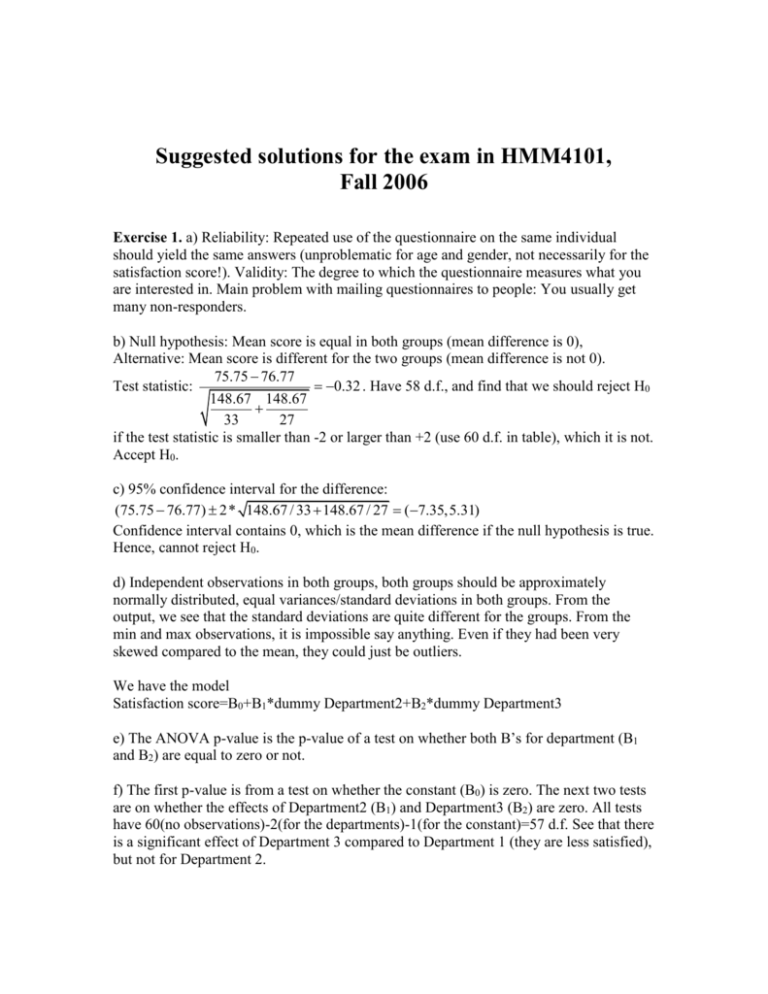
Suggested solutions for the exam in HMM4101,
Fall 2006
Exercise 1. a) Reliability: Repeated use of the questionnaire on the same individual
should yield the same answers (unproblematic for age and gender, not necessarily for the
satisfaction score!). Validity: The degree to which the questionnaire measures what you
are interested in. Main problem with mailing questionnaires to people: You usually get
many non-responders.
b) Null hypothesis: Mean score is equal in both groups (mean difference is 0),
Alternative: Mean score is different for the two groups (mean difference is not 0).
75.75  76.77
 0.32 . Have 58 d.f., and find that we should reject H0
Test statistic:
148.67 148.67

33
27
if the test statistic is smaller than -2 or larger than +2 (use 60 d.f. in table), which it is not.
Accept H0.
c) 95% confidence interval for the difference:
(75.75  76.77)  2* 148.67 / 33  148.67 / 27  (7.35,5.31)
Confidence interval contains 0, which is the mean difference if the null hypothesis is true.
Hence, cannot reject H0.
d) Independent observations in both groups, both groups should be approximately
normally distributed, equal variances/standard deviations in both groups. From the
output, we see that the standard deviations are quite different for the groups. From the
min and max observations, it is impossible say anything. Even if they had been very
skewed compared to the mean, they could just be outliers.
We have the model
Satisfaction score=B0+B1*dummy Department2+B2*dummy Department3
e) The ANOVA p-value is the p-value of a test on whether both B’s for department (B1
and B2) are equal to zero or not.
f) The first p-value is from a test on whether the constant (B0) is zero. The next two tests
are on whether the effects of Department2 (B1) and Department3 (B2) are zero. All tests
have 60(no observations)-2(for the departments)-1(for the constant)=57 d.f. See that there
is a significant effect of Department 3 compared to Department 1 (they are less satisfied),
but not for Department 2.
g) Mean score for Department 1 is 81.46. Difference in score between Dept’s 2 and 3 is
0.29-(-17.90)=18.19 (or, 81.46+0.29*1-(81.46-17.90*1)=18.19). Since there is no
significant difference between Dept’s 1 and 2, might want to collapse these two
categories.
h) 95% confidence interval (have to use 2.5% and 97.5% percentiles from t-distribution
with 60 d.f. which is +/-2): 0.188  2*0.08  (0.35, 0.03) . Popular, somewhat
incorrect interpretation (1p) is that we can be 95% sure that the true regression
coefficient, or the slope of the regression line, lies within this interval. The correct
interpretation (2p) is that if we repeat the study with 60 patients many times, the
unknown, true regression coefficient will lie within this interval in 95% of the studies.
i) Since the effect of age changes from significant to non-significant, while the effect for
department is almost unchanged, department is the confounder. From the univariate
analysis of age, we see that older people appear to score lower on satisfaction. From the
analysis of department, we know that patients in department 3 score lower on
satisfaction. From the multivariate analysis, we know that department is the important
variable, not age. Hence, department 3 has to have older patients than the other two
departments, and this creates the imaginary effect of age in the univariate analysis.
j) If continuous: One-way ANOVA or Kruskal-Wallis. If categorical: Chi-square test.
Advantages/Disadvantages: Here I wanted you to say something about test power
(perhaps a bit difficult). In order to do ANOVA you need normally distributed pain
scores. You do not need this assumption for Kruskal-Wallis or Chi-square. However, if
the pain scores are normal, then you loose a lot of power if you use the categorical
coding/Chi-square test (need more data to get significant results). If the data are not
normal, you would still loose some power by using categorical coding/Chi-square
compared to continuous coding/Kruskal-Wallis (one-way ANOVA is irrelevant in this
case, as the assumptions for it are not fulfilled). Hence, you loose information and power
if you transform the continuous pain score to categorical scores. However, you do not
need to check if the data are normal or not if you use the categorical coding.
Exercise 2. a) Null hypothesis: The proportions of cured individuals are the same in both
groups. Alternative: The proportions are different. In order to calculate the test statistic,
30*0.7  30*0.5
 0.6
we need the common proportion (see p. 382 in textbook):
60
0.7  0.5
 1.58 . The test statistic is approximately
Test statistic:
0.6*(1  0.6) 0.6*(1  0.6)

30
30
standard normal, and should be compared to the 0.025% and 97.5% percentiles of the
standard normal distribution, +/-1.96. Hence, the conclusion is that the new medicine is
not significantly better than the competition (in Norway, this would mean that the new
medicine would not be marketed). You can get the same conclusion if you use a Chisquare test instead!!
b) The number of cured individuals can be called successes, and follow a binomial
distribution. You have 30 independent trials in each group, two possible outcomes
(cured/not cured) and the probability of being cured can be considered to be the same for
each individual in each group. The reason why you still end up with a test based on the
normal distribution, is because of the central limit theorem. If you have many
observations, from any distribution without “extreme” values, you end up with something
that is standard normal if you subtract the expected value and divide by the standard
error.
c) Probability that a random individual does not get the side effect: 1-1/5000 (by the
complement rule). Probability that none out of 2000 individuals get the side effect: (11/5000)2000=0.67=67%, if you assume that the individuals are independent.