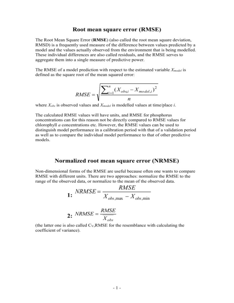
Root mean square error (RMSE)
The Root Mean Square Error (RMSE) (also called the root mean square deviation,
RMSD) is a frequently used measure of the difference between values predicted by a
model and the values actually observed from the environment that is being modelled.
These individual differences are also called residuals, and the RMSE serves to
aggregate them into a single measure of predictive power.
The RMSE of a model prediction with respect to the estimated variable Xmodel is
defined as the square root of the mean squared error:
RMSE 

n
i 1
( X obs,i  X mo del ,i ) 2
n
where Xobs is observed values and Xmodel is modelled values at time/place i.
The calculated RMSE values will have units, and RMSE for phosphorus
concentrations can for this reason not be directly compared to RMSE values for
chlorophyll a concentrations etc. However, the RMSE values can be used to
distinguish model performance in a calibration period with that of a validation period
as well as to compare the individual model performance to that of other predictive
models.
Normalized root mean square error (NRMSE)
Non-dimensional forms of the RMSE are useful because often one wants to compare
RMSE with different units. There are two approaches: normalize the RMSE to the
range of the observed data, or normalize to the mean of the observed data.
1:
NRMSE 
RMSE
X obs ,max  X obs ,min
RMSE
NRMSE

2:
X obs
(the latter one is also called CV,RMSE for the resemblance with calculating the
coefficient of variance).
-1-
Pearson correlation coefficient (r)
Correlation – often measured as a correlation coefficient – indicates the strength and
direction of a linear relationship between two variables (for example model output
and observed values). A number of different coefficients are used for different
situations. The best known is the Pearson product-moment correlation coefficient
(also called Pearson correlation coefficient or the sample correlation coefficient),
which is obtained by dividing the covariance of the two variables by the product of
their standard deviations. If we have a series n observations and n model values, then
the Pearson product-moment correlation coefficient can be used to estimate the
correlation between model and observations.
r


n
i 1
n
i 1
( xi  x)  ( yi  y )
( xi  x) 2 

n
i 1
( yi  y ) 2
The correlation is +1 in the case of a perfect increasing linear relationship, and -1 in
case of a decreasing linear relationship, and the values in between indicates the degree
of linear relationship between for example model and observations. A correlation
coefficient of 0 means the there is no linear relationship between the variables.
The square of the Pearson correlation coefficient (r2), known as the coefficient of
determination, describes how much of the variance between the two variables is
described by the linear fit.
-2-
Nash-Sutcliffe coefficient (E)
The Nash-Sutcliffe model efficiency coefficient (E) is commonly used to assess the
predictive power of hydrological discharge models. However, it can also be used to
quantitatively describe the accuracy of model outputs for other things than discharge
(such as nutrient loadings, temperature, concentrations etc.). It is defined as:
n
( X obs,i  X mo del ) 2
i 1
E  1


n
( X obs,i  X obs ) 2
i 1
where Xobs is observed values and Xmodel is modelled values at time/place i.
Nash-Sutcliffe efficiencies can range from - to 1. An efficiency of 1 (E = 1)
corresponds to a perfect match between model and observations. An efficiency of 0
indicates that the model predictions are as accurate as the mean of the observed data,
whereas an efficiency less than zero (- < E < 0) occurs when the observed mean is a
better predictor than the model.
Essentially, the closer the model efficiency is to 1, the more accurate the model is.
-3-