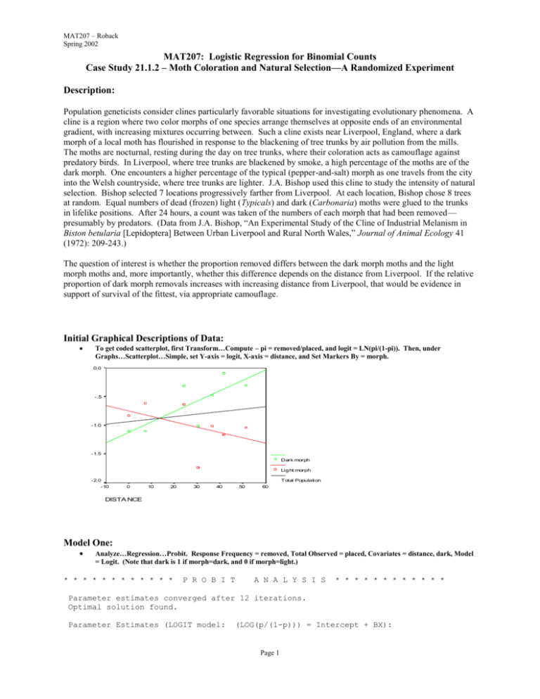
MAT207 – Roback
Spring 2002
MAT207: Logistic Regression for Binomial Counts
Case Study 21.1.2 – Moth Coloration and Natural Selection—A Randomized Experiment
Description:
Population geneticists consider clines particularly favorable situations for investigating evolutionary phenomena. A
cline is a region where two color morphs of one species arrange themselves at opposite ends of an environmental
gradient, with increasing mixtures occurring between. Such a cline exists near Liverpool, England, where a dark
morph of a local moth has flourished in response to the blackening of tree trunks by air pollution from the mills.
The moths are nocturnal, resting during the day on tree trunks, where their coloration acts as camouflage against
predatory birds. In Liverpool, where tree trunks are blackened by smoke, a high percentage of the moths are of the
dark morph. One encounters a higher percentage of the typical (pepper-and-salt) morph as one travels from the city
into the Welsh countryside, where tree trunks are lighter. J.A. Bishop used this cline to study the intensity of natural
selection. Bishop selected 7 locations progressively farther from Liverpool. At each location, Bishop chose 8 trees
at random. Equal numbers of dead (frozen) light (Typicals) and dark (Carbonaria) moths were glued to the trunks
in lifelike positions. After 24 hours, a count was taken of the numbers of each morph that had been removed—
presumably by predators. (Data from J.A. Bishop, “An Experimental Study of the Cline of Industrial Melanism in
Biston betularia [Lepidoptera] Between Urban Liverpool and Rural North Wales,” Journal of Animal Ecology 41
(1972): 209-243.)
The question of interest is whether the proportion removed differs between the dark morph moths and the light
morph moths and, more importantly, whether this difference depends on the distance from Liverpool. If the relative
proportion of dark morph removals increases with increasing distance from Liverpool, that would be evidence in
support of survival of the fittest, via appropriate camouflage.
Initial Graphical Descriptions of Data:

To get coded scatterplot, first Transform…Compute – pi = removed/placed, and logit = LN(pi/(1-pi)). Then, under
Graphs…Scatterplot…Simple, set Y-axis = logit, X-axis = distance, and Set Markers By = morph.
0.0
-.5
-1.0
-1.5
LOGIT
Dark morph
Lig ht morph
-2.0
Total Population
-10
0
10
20
30
40
50
60
DISTA NCE
Model One:

Analyze…Regression…Probit. Response Frequency = removed, Total Observed = placed, Covariates = distance, dark, Model
= Logit. (Note that dark is 1 if morph=dark, and 0 if morph=light.)
* * * * * * * * * * * *
P R O B I T
A N A L Y S I S
* * * * * * * * * * * *
Parameter estimates converged after 12 iterations.
Optimal solution found.
Parameter Estimates (LOGIT model:
(LOG(p/(1-p))) = Intercept + BX):
Page 1
MAT207 – Roback
Spring 2002
Regression Coeff.
DISTANCE
DARK
Pearson
Standard Error
Coeff./S.E.
.00531
.40405
.00400
.13938
1.32792
2.89895
Intercept
Standard Error
Intercept/S.E.
-1.13674
.15676
-7.25156
Goodness-of-Fit
Chi Square =
24.798
DF = 11
P =
.010
Since Goodness-of-Fit Chi square is significant, a heterogeneity
factor is used in the calculation of confidence limits.
Observed and Expected Frequencies
DISTANCE
Number of
Subjects
Observed
Responses
Expected
Responses
Residual
Prob
.00
.00
7.20
7.20
24.10
24.10
30.20
30.20
36.40
36.40
41.50
41.50
51.20
51.20
56.0
56.0
80.0
80.0
52.0
52.0
60.0
60.0
60.0
60.0
84.0
84.0
92.0
92.0
17.0
14.0
28.0
20.0
18.0
22.0
9.0
16.0
16.0
23.0
20.0
40.0
24.0
39.0
13.603
18.178
20.002
26.644
13.896
18.371
16.418
21.644
16.814
22.101
24.001
31.474
27.266
35.589
3.397
-4.178
7.998
-6.644
4.104
3.629
-7.418
-5.644
-.814
.899
-4.001
8.526
-3.266
3.411
.24292
.32460
.25002
.33305
.26724
.35329
.27363
.36073
.28023
.36836
.28573
.37469
.29636
.38684
Model Two:

Analyze…Regression…Probit. Response Frequency = removed, Total Observed = placed, Covariates = distance, dark,
drkbydst; Model = Logit. (Note that drkbydst=dark*distance.)
* * * * * * * * * * * *
P R O B I T
A N A L Y S I S
* * * * * * * * * * * *
Parameter estimates converged after 13 iterations.
Optimal solution found.
Parameter Estimates (LOGIT model:
Regression Coeff.
DISTANCE
DARK
DRKBYDST
Pearson
(LOG(p/(1-p))) = Intercept + BX):
Standard Error
Coeff./S.E.
-.00929
-.41126
.02779
.00579
.27449
.00809
-1.60439
-1.49826
3.43691
Intercept
Standard Error
Intercept/S.E.
-.71773
.19020
-3.77345
Goodness-of-Fit
Chi Square =
12.709
DF = 10
P =
.240
Since Goodness-of-Fit Chi square is NOT significant, no heterogeneity
factor is used in the calculation of confidence limits.
Page 2
MAT207 – Roback
Spring 2002
Observed and Expected Frequencies
DISTANCE
Number of
Subjects
Observed
Responses
Expected
Responses
Residual
Prob
.00
.00
7.20
7.20
24.10
24.10
30.20
30.20
36.40
36.40
41.50
41.50
51.20
51.20
56.0
56.0
80.0
80.0
52.0
52.0
60.0
60.0
60.0
60.0
84.0
84.0
92.0
92.0
17.0
14.0
28.0
20.0
18.0
22.0
9.0
16.0
16.0
23.0
20.0
40.0
24.0
39.0
18.362
13.683
25.066
21.582
14.591
17.450
16.158
21.671
15.487
23.283
20.929
34.497
21.407
41.833
-1.362
.317
2.934
-1.582
3.409
4.550
-7.158
-5.671
.513
-.283
-.929
5.503
2.593
-2.833
.32789
.24435
.31333
.26977
.28059
.33557
.26930
.36119
.25812
.38805
.24915
.41068
.23268
.45471
Model Three:

Analyze…Regression…Probit. Response Frequency = removed, Total Observed = placed, Factor = loca_int, Covariates =
dark, drkbydst; Model = Logit. (Note that loca_int takes on values 1-7 corresponding to the 7 sites.)
* * * * * * * * * * * *
LOCA_INT
Level
1
2
3
4
5
6
7
P R O B I T
N of Cases
2
2
2
2
2
2
2
A N A L Y S I S
* * * * * * * * * * * *
Label
1
2
3
4
5
6
7
Parameter estimates converged after 18 iterations.
Optimal solution found.
Parameter Estimates (LOGIT model:
Regression Coeff.
DARK
DRKBYDST
Pearson
(LOG(p/(1-p))) = Intercept + BX):
Standard Error
Coeff./S.E.
-.40546
.02774
.27519
.00810
-1.47341
3.42574
Intercept
Standard Error
Intercept/S.E.
LOCA_INT
-.76692
-.74655
-.60353
-1.56475
-1.04906
-.98067
-1.20122
.24621
.20418
.21575
.23933
.21431
.18966
.20768
-3.11485
-3.65636
-2.79736
-6.53806
-4.89501
-5.17060
-5.78397
1
2
3
4
5
6
7
Goodness-of-Fit
Chi Square =
2.867
DF = 5
P =
.720
Since Goodness-of-Fit Chi square is NOT significant, no heterogeneity
factor is used in the calculation of confidence limits.
Page 3
MAT207 – Roback
Spring 2002
Observed and Expected Frequencies
LOCA_INT
DARK
Number of
Subjects
Observed
Responses
Expected
Responses
Residual
Prob
1
1
.00
1.00
56.0
56.0
17.0
14.0
17.760
13.240
-.760
.760
.31715
.23642
2
2
.00
1.00
80.0
80.0
28.0
20.0
25.726
22.274
2.274
-2.274
.32157
.27843
3
3
.00
1.00
52.0
52.0
18.0
22.0
18.384
21.616
-.384
.384
.35354
.41569
4
4
.00
1.00
60.0
60.0
9.0
16.0
10.378
14.622
-1.378
1.378
.17297
.24370
5
5
.00
1.00
60.0
60.0
16.0
23.0
15.564
23.436
.436
-.436
.25941
.39059
6
6
.00
1.00
84.0
84.0
20.0
40.0
22.912
37.088
-2.912
2.912
.27276
.44153
7
7
.00
1.00
92.0
92.0
24.0
39.0
21.276
41.724
2.724
-2.724
.23126
.45352
Page 4