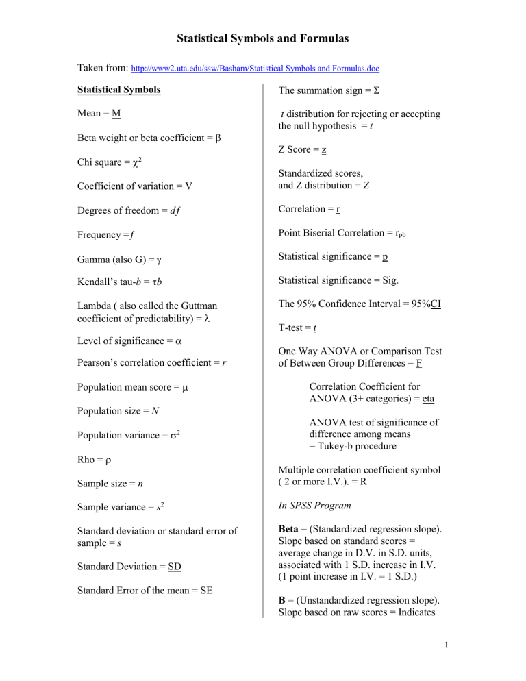
Statistical Symbols and Formulas
Taken from: http://www2.uta.edu/ssw/Basham/Statistical Symbols and Formulas.doc
Statistical Symbols
The summation sign = 
Mean = M
t distribution for rejecting or accepting
the null hypothesis = t
Beta weight or beta coefficient = 
Z Score = z
Chi square = 
2
Coefficient of variation = V
Standardized scores,
and Z distribution = Z
Degrees of freedom = d
Correlation = r
Frequency =
Point Biserial Correlation = rpb
Gamma (also G) = 
Statistical significance = p
Kendall’s tau-b = b
Statistical significance = Sig.
Lambda ( also called the Guttman
coefficient of predictability) = 
The 95% Confidence Interval = 95%CI
T-test = t
Level of significance = 
Pearson’s correlation coefficient = r
Population mean score = 
One Way ANOVA or Comparison Test
of Between Group Differences = F
Correlation Coefficient for
ANOVA (3+ categories) = eta
Population size = N
Population variance = 
2
ANOVA test of significance of
difference among means
= Tukey-b procedure
Rho = 
Sample size = n
Multiple correlation coefficient symbol
( 2 or more I.V.). = R
Sample variance = s2
In SPSS Program
Standard deviation or standard error of
sample = s
Beta = (Standardized regression slope).
Slope based on standard scores =
average change in D.V. in S.D. units,
associated with 1 S.D. increase in I.V.
(1 point increase in I.V. = 1 S.D.)
Standard Deviation = SD
Standard Error of the mean = SE
B = (Unstandardized regression slope).
Slope based on raw scores = Indicates
1
Statistical Symbols and Formulas
average change in D.V. for 1 point
increase in I.V.
 = Beta weight or beta coefficient
Variance Measures in a Population
(Simple Distribution and Frequency
Distribution)
R2 change = tells whether or not variables
entered at that point add anything over
and above variables that have been
added previously.
Population Standard Deviation
___
 =  2 , or
Variance =  X2
 X   X2
Covariance (of x and y) =  XY
(Simple Distribution)
Statistical Formulas
Population Variance
Measures of Central Tendency
2 = 1( X2 – ( X )2
N–1
(Simple Distribution)
(Frequency Distribution)
Mean =  =  
N
Population Mean =  X  X 
Population Variance
1 n
 Xi
n i 1
2 = 1 ( fX2 – ( fX )2
N
N–1
(Frequency Distribution)
Variance =
Mean =  =  f 
N
Sum of squared distributions from the mean for all cases
(number of cases –1)
or,
Mdn = simple distribution = center score
odd population
Mdn = simple distribution =
Even population
2 center scores divided by 2
(X-M)2
N–1
Note:
col:[X M X-M (X-M)2] (X-M)2
N–1
or,
Mdn = frequency distribution =
LRL – (PN-CFL .h)
FI
X 
1  n 2 1  n

 X i    X i 
n  i 1
n  i 1 
2



Mode = Most Frequent Score
2
Statistical Symbols and Formulas
Variance Measures in a Sample
(Simple Distribution and Frequency
Distribution)
Standard Error of The Mean Formula:
SEM = SD
N–1
Population Standard Deviation
___
s =  s2
Confidence Interval at 95% Formula:
(Simple Distribution)
Calculating Percent Formula:
Sample Variance
3 x X = 3x100 = 300/6 = x = 50
6 100
s2 = 1( x2 – ( x )2
n–1
(Frequency Distribution)
M + (1.96)(SEM)
Z Statistic Formula:
Z=M-
m
Sample Variance
s2 = 1 ( fx2 – ( fx )2
n
n–1
 m = SD
 N –1
t-test Statistic Formula:
Statistical Average Formula:
M + 1 = Mean + 1 Standard Deviation
t = M1 – M2
SE diff
Raw Score Transformation Formula:
Confidence Interval for t-test Formula:
Z Standard Scores
CI = M1 – M2 + (?) (SE diff)
scores – mean = X - M
standard deviation

Point Biserial Correlation Coefficient:
________________
Probability Density Formula:
M + 1SD = 68%
M + 1.96SD = 95%
Coefficient of Variation Formula:
Coefficient of Variation = SD x 100
Mean
rpb =  _____t2_______
t2 + ( n1 + n2 – 2)
Note: Used for t test for independent groups
Eta Correlation Coefficient Formula:
(for ANOVA 3+ Categories)
eta2 = SS Between / SS Total, or
 between = eta2
 total
____
3
Statistical Symbols and Formulas
eta =  eta2
Formula for Characterizing a Straight
Line:
D Index Calculation Formula:
(Measure of effect size)
y = a + Bx
Difference between 2 group means
Avg. SD of the 2 groups
y = Predicted value of Dependent
Variable (D.V.)
a = Intercept value of D.V. when
the Independent Variable (I.V.) =
0
B = Slope = Average change of
D.V. associated with a 1 point
increase in the I.V.
x = Value of I. V.
Note: Used in Meta Analysis
(or SD of Control group)
Note: less accurate
Formula for Calculating Covariance of
two variables (x and y):
Covariance =  XY
Residual = for a particular person their
actual value minus their predicted value.
Therefore,
 XY 
1 n
1 n
 n  
X
Y

X
Yi  
 i i
 i  
n  i 1
n  i 1 
i 1

The coefficient of correlation of X an Y
is then stated as:  XY
Then to get a better measure of
correlation calculate:
Formula for Calculating a Residual:
Residual = D.V. – y
Residual = actual value of D.V. –
predicted value.
Conversion Formula for Standard
Scores: Bivariate
Value of I.V.
_
-Mean of I.V. or, z = x - x
 S.D. of I.V.
S.D. x
1 n
 n 
X iYi    X i    Yi 

n  i 1   i 1 
i 1
n
 XY 
2
2
 n 2 1  n
   n 2 1  n  
 X i    X i    Yi    Yi  
n  i 1    i 1
n  i 1  
 i 1
Formula for Calculating
Covariance Matrix:
 2
C X
 XY
a
2x2
Formula for a Bivariate Normal
Distribution:
4


0
0
 
 XY 

 Y2 
Formula for Calculating the Eigenvalues
of the Covariance Matrix:
p     det  I  C 
Note: Does not change shape of distribution.
 
 XY
2
X
 XY
   Y2
e ( x
2
 y2 )
dx dy  1
Formula for Calculating the Slope of a
Regression Line:
ˆ  
X iYi  nX Y
X
2
i
 nX 2
4
Statistical Symbols and Formulas
Multivariate Interaction Effects
Multivariate ANCOVA (Computation
Formula:
formula for adjusted means):
Computation formula for data points
= Y=a+X1(pre)B(pre) + X2(group)B(group)
Y=a+X1B1 + X2B2 + X12B12
Example:
Yd=a+Xagbag + Xincbinc + X(ag)(inc)b(ag)(inc)
Constant = a
Unit of associated change =1, or
0 =X
Predicted value of 1st slope = bag
Predicted value of 2nd slope = binc
Predicted value of score = Y
Spearman Correlation Formula:
rs = 1- 6D2
n(n2 – 1)
Pearson Correlation Formula:
r = _SP_
SSxSSy
Intercept Constant = a
Descriptive mean of pretest
condition = X1
Unit of associated change
=Experimental group =1, or
Control group =0 =X2
Predicted value of 1st slope =
B(pre)
In Bivariate regression only: ( see SPSS
symbol definitions below).
Beta = r  B, or
Beta = r
Note: r  B
Predicted value of 2nd slope = B
(post)
Predicted value of score = Y
adjusted experimental mean =
Y
adjusted control mean =
__
__
where SP =  (X – X)(Y – Y) =
Logistic Regression Odds Ratio
XY - (X) (Y)
n
Formula:
100 (OR – 1) = % Change
Partial Correlation Ratio Formula:
r2 = a
a+d
(i.e. 100 (.5 – 1) = 50% decrease in odds
of participation)
Chi-Square Statistic Formula:
Part Correlation Ratio Formula:
r2 = a
a+b+c+d
2 =  ( o - e)2
e
5
Statistical Symbols and Formulas
To be continued …
6