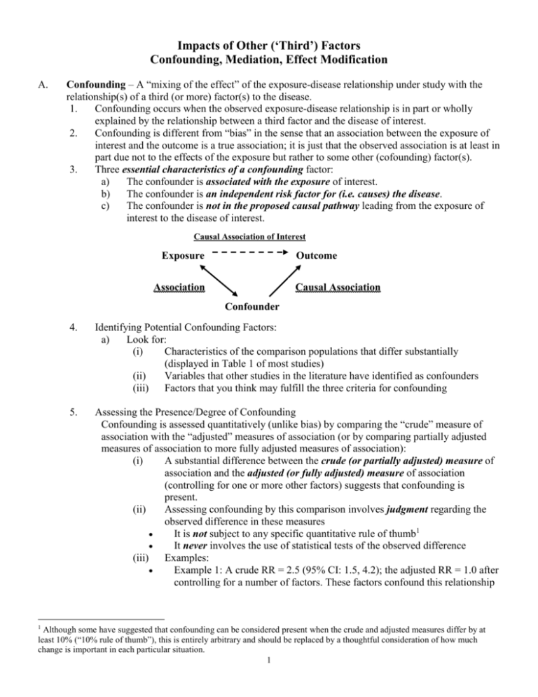
Impacts of Other (‘Third’) Factors
Confounding, Mediation, Effect Modification
A.
Confounding – A “mixing of the effect” of the exposure-disease relationship under study with the
relationship(s) of a third (or more) factor(s) to the disease.
1.
Confounding occurs when the observed exposure-disease relationship is in part or wholly
explained by the relationship between a third factor and the disease of interest.
2.
Confounding is different from “bias” in the sense that an association between the exposure of
interest and the outcome is a true association; it is just that the observed association is at least in
part due not to the effects of the exposure but rather to some other (cofounding) factor(s).
3.
Three essential characteristics of a confounding factor:
a)
The confounder is associated with the exposure of interest.
b)
The confounder is an independent risk factor for (i.e. causes) the disease.
c)
The confounder is not in the proposed causal pathway leading from the exposure of
interest to the disease of interest.
Causal Association of Interest
Exposure
Outcome
Association
Causal Association
Confounder
1
4.
Identifying Potential Confounding Factors:
a)
Look for:
(i)
Characteristics of the comparison populations that differ substantially
(displayed in Table 1 of most studies)
(ii)
Variables that other studies in the literature have identified as confounders
(iii) Factors that you think may fulfill the three criteria for confounding
5.
Assessing the Presence/Degree of Confounding
Confounding is assessed quantitatively (unlike bias) by comparing the “crude” measure of
association with the “adjusted” measures of association (or by comparing partially adjusted
measures of association to more fully adjusted measures of association):
(i)
A substantial difference between the crude (or partially adjusted) measure of
association and the adjusted (or fully adjusted) measure of association
(controlling for one or more other factors) suggests that confounding is
present.
(ii)
Assessing confounding by this comparison involves judgment regarding the
observed difference in these measures

It is not subject to any specific quantitative rule of thumb1

It never involves the use of statistical tests of the observed difference
(iii) Examples:

Example 1: A crude RR = 2.5 (95% CI: 1.5, 4.2); the adjusted RR = 1.0 after
controlling for a number of factors. These factors confound this relationship
Although some have suggested that confounding can be considered present when the crude and adjusted measures differ by at
least 10% (“10% rule of thumb”), this is entirely arbitrary and should be replaced by a thoughtful consideration of how much
change is important in each particular situation.
1



to the extent that they completely explain the observed (crude) exposuredisease relationship
Example 2: A crude RR = 2.5 (95% CI: 1.5, 4.2); the adjusted RR = 2.0
(95% CI: 1.1, 3.4) after controlling for a number of factors. These factors
modestly confound (partially explain) this relationship, though the adjusted
(un-confounded) exposure-disease relationship is still statistically
significant.
Example 3: A crude RR = 2.5 (95% CI: 1.5, 4.2); the adjusted RR = 3.5
(95% CI: 2.2, 5.4) after controlling for a number of factors. These factors
confound this relationship but in the opposite direction (this can occur when
either the confounding factor is a protective factor rather than a risk factor,
or when the confounding factor is negatively associated with the exposure of
interest)
Example 4: A crude RR = 0.40 (95% CI: 0.15, 0.75); the adjusted RR = 0.65
(95% CI: 0.40, 1.2) after controlling for a number of factors. These factors
confound (at least partially explain) the relationship; the remaining adjusted
relationship is no longer statistically significant.
6.
Methods for Preventing Confounding in Study Design
a)
Restricting the study subjects to only one category or level of a particularly critical
confounding factor (e.g. a narrow age range or to women only).
b)
Matching subject on important potential confounder(s); assures that comparison groups
are the same
c)
Randomizing (intervention/RCT only); an attempt to produce comparison groups that
are similar on both known and unknown confounders.
7.
Methods for Correcting Confounding in the Analysis
a)
Stratification (report and compare findings for each category or at each level of the
confounding factor); this should decrease or eliminate confounding effects by the
stratifying factor.
b)
Standardization or adjustment for an important confounding factor
c)
Multiple regression to “adjust” for multiple confounding factors
d)
Left-Over Confounding: Even after controlling for multiple factors, remember that
some left-over confounding may still be present because:
(i)
Unknown Confounding: the analysis cannot control for factors that have not
been measured (didn’t think of them or didn’t collect data on them); those
unmeasured factors could act as confounders
(ii)
Residual Confounding: one or more confounders may be poorly/imprecisely
measured; to the extent that this happens the analysis will leave some left-over
(“residual”) confounding unaccounted for. Improving the measurement of
confounders would help eliminate this source of additional confounding.
8.
Evaluating Confounding
a)
What was the observed effect of confounding in the study?
b)
Did the study identify and control for all of the important known confounders, i.e. are
there confounders not accounted for?
c)
Did the study measure and model the confounders appropriately, i.e. is can you identify
any possibility of residual confounding?
d)
What is the potential that there are unknown confounders still confounding the
relationship?
2
B.
Mediation – occurs when the measured association between the exposure and the outcome is
mediated by one or more other factors
1.
2.
C.
These factors, like confounders, are associated with the exposure and cause the outcome, but
they are, by definition, in the causal pathway
We may adjust for these factors (as for confounders) to indicate how much of the association
between exposure and outcome is related to causal mechanisms involving the mediator.
Effect Measure Modification – occurs when the measured association between the exposure and the
event/disease under study varies by levels of a third factor (i.e. when the measure of the “effect” the
exposure has on the outcome (the “effect measure”) is “modified” by varying levels of a third factor)
1.
2.
Presence of effect modification is determined by examining the exposure-event/disease
relationship in the different strata of the third factor of interest, either exposed/unexposed (e.g.
gender) or different levels of exposure (e.g. age, SES)
a)
With confounding, the exposure-event/disease relationship (measure of association or
effect measure) is similar in different strata (and different from the crude relationship)

For example, a crude exposure-event RR = 1.6 with a gender adjusted RR =
1.0 (>10% change) and category specific RR estimates of 1.1 and 0.95 for
males and females respectively. Because the category specific estimates are
close to one another, combining them into an overall gender-adjusted
estimate is perfectly appropriate.
b)
With effect modification, the exposure-event/disease relationship (measure of
association or effect measure) is different in different strata of the third factor.

For example, a crude exposure-event RR = 1.6 with a gender adjusted RR =
1.0 (>10% change) but category specific RR estimates of 1.5 and 0.75 for
males and females respectively. Because the category specific estimates are
very different (suggesting the exposure is a risk factor for males but
protective for women), combining them into an overall gender-adjusted
estimate is not appropriate (because it hides very important information
about what is going on in the exposure-event relationship, information you
would want to report not hide!)
Assessing effect modification involves examining the exposure-event/disease relationship
across different strata of the third variable. It is done in two ways:
a)
“Eyeball” the data to make a qualitative judgment about the pattern of variation in
exposure-event/disease relationship across different strata
b)
Use one of the chi-square tests for “homogeneity” (or “heterogeneity”) to assess the
uniformity of estimates across strata

These chi-square methods test the null hypothesis that the degree of
variability in the stratum-specific estimates is consistent with random
variation (thus rejecting the null hypothesis, with p-values <0.05, suggests
that the estimates are not homogeneous and should not be combined; failing
to reject the null hypothesis suggests that the estimates are homogeneous
enough to combine into an overall adjusted measure of association).

Statistical tests do not replace the need to make judgments about the
observed variation
3