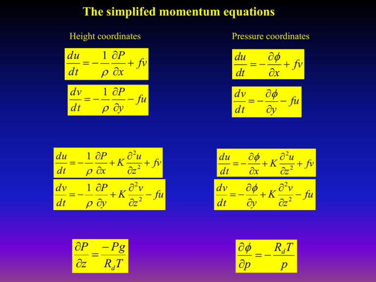
The simplifed momentum equations
Height coordinates
Pressure coordinates
du
1 P

 fv
dt
 x
du


 fv
dt
x
dv
1 P

 fu
dt
 y
dv


 fu
dt
y
du
1 P
 2u

 K 2  fv
dt
 x
z
du

 2u

 K 2  fv
dt
x
z
dv
1 P
 2v

 K 2  fu
dt
 y
z
dv

 2v

 K 2  fu
dt
y
z
P  Pg

z Rd T
RT

 d
p
p
In this section we will derive the four most important
relationships describing atmospheric structure
1. Hydrostatic Balance: the vertical force balance in the
atmosphere
2. The Hypsometric Equation: the relationship between the
virtual temperature of a layer and the layer’s thickness
3. Geostrophic Balance: the most fundamental horizontal
force balance in the atmosphere
4. Thermal wind Balance: a relationship between the wind at
an upper level of the atmosphere and the temperature
gradient below that level
We will then expand our understanding of balanced
flow to include more complicated force balances in
horizontal flows
1. Geostrophic Flow: the flow resulting from a balance
between the PGF and Coriolis force in straight flow
2. Inertial Flow: curved flow resulting when the Coriolis
force balances the “Centrifugal” force
3. Cyclostrophic Flow: Flow that results when the pressure
gradient force balances the Centrifugal force
4. Gradient flow: Flow that results when the pressure
gradient force and Coriolis force balance the Centrifugal
force
Virtual Temperature:
The temperature that a parcel of dry air
would have if it were at the same pressure and had the same density
as moist air.
P = pressure
d = dry air density
Derivation:
Start with ideal gas law for moist air:
P  RT
P  d Rd T  v RvT
v = vapor density
= air density
R= gas constant
Rv = vapor gas constant
Rd = dry air gas constant
T = Temperature
Now treat moist air as if it were dry by introducing the virtual temperature Tv
P  d Rd  v Rv T  d  v Rd Tv  Rd Tv
What is the relationship between the temperature, T
And the virtual temperature Tv?
d Rd  v Rv T  d  v RdTv
Write:
M

V
Mv 
 Md
 Md Mv 
Rd 
Rv T  


 Rd Tv
V
V 
 V

 V
M = mass of air
Md = mass of dry air
Mv = mass of vapor
V = volume
Multiply and divide second term by Rd
 Md
M v Rd Rv 
 Md Mv 

T  
Rd 

 Rd Tv
V Rd 
V 
 V
 V
Cancel Rd and rearrange
 M d M v Rv


V
V Rd

Tv 
 Md Mv
 V  V



T



From last page:
 M d M v Rv


V
V Rd
Tv  
 Md Mv
 V  V



T



Cancel V, and divide top and bottom terms by Md:
M v Rv

1
M d Rd

Tv 

Mv
 1 M
d



T



Introduce mixing ratio: rv = Mv/Md and let e = Rd/Rv

1
 1  rv   
 e  T
Tv  
 1  rv 




From last page:

1
 1  rv   
 e  T
Tv  
 1  rv 




Approximate (1+rv)-1 = 1- rv and use 1/e = 1.61


Tv  1  rv 1 1.61rv T  1  rv 1.61rv 1.61rv2 T
Neglect rv2 term
Tv  1 0.61rv T
HYDROSTATIC BALANCE
0
1 P
g
 z
The atmosphere is in hydrostatic
balance essentially everywhere
except in core regions of significant
storms such as hurricanes and
thunderstorms
The Hypsometric Equation
Consider a column of atmosphere
that is 1 m by 1 m in area and
extends from sea level to space
Let’s isolate the part of this
column that extends between the
1000 hPa surface and the 500 hPa
surface
How much mass is in the column?
 100 N m 2 


1
 1 m 2  
  5102.04 kg
Mass  (1000 500) hPa 
2 
 9.81 m s 
 hPa 
How thick is the column? That depends…………
P
  g
z
Hydrostatic equation
p  Rd Tv
Ideal Gas Law
Substitute ideal gas law into hydrostatic equation
Rd Tv p
z  
g p
Integrate this equation between two levels (p2, z2) and (p1, z1)
z2
Rd Tv p
g p
p1
p2
 z   
z1
Rd Tv p
g p
p1
z2
p2
 z   
z1
z2
 z 
z1
From previous page
p1
Rd Tv
p g  ln p
2
Problem: Tv varies with altitude. To perform the integral
on the right we have to consider the pressure weighted
column average virtual temperature given by:
We can then integrate to give
p1
 T  ln p
v
Tv 
p2
p1
  ln p
p2
Rd Tv  p1 
z 2  z1 
ln 
g
 p2 
This equation is called the Hypsometric Equation
The equation relates the thickness of a layer of air between two
pressure levels to the average virtual temperature of the layer
Geopotential Height
We can express the hypsometric (and hydrostatic) equation in terms
of a quantity called the geopotential height
Geopotential (): Work (energy) required to raise a unit mass a
distance dz above sea level
d  gdz
 p1 
  Rd Tv ln 
 p2 
Meteorologists often refer to “geopotential height” because this quantity is directly
associated with energy to vertically displace air
Geopotential Height (Z):
Z
 gz

g0 g0
g0 is the globally averaged
Value of gravity at sea level
For practical purposes, Z and z are about the same in the troposphere
Atmospheric pressure varies exponentially with altitude, but very slowly on
a horizontal plane – as a result, a map of surface (station) pressure looks like
a map of altitude above sea level.
variation of pressure
with altitude
observed surface pressure
over central North America
Station pressures are measured at locations worldwide
Analysis of horizontal pressure fields, which are responsible for
the earth’s winds and are critical to analysis of weather systems,
requires that station pressures be converted to a common level,
which, by convention, is mean sea level.
Reduction of station pressure to sea level pressure:
0
Integrate hypsometric equation
dp
g
p p  z  RTv dz (4)
sea level pressure (PSL)
to station pressure (PSTN)
g
and right side from z = 0
ln pSL   ln pSTN  
zSTN (5)
to station altitude (ZSTN).
Rd Tv
p SL
STA
STA
BUT WHAT IS Tv? WE HAVE ASSUMED A FICTICIOUS
ATMOSPHERE THAT IS BELOW GROUND!!!
National Weather Service Procedure to estimate Tv
1. Assume Tv = T
2. Assume a mean surface temperature = average of
current temperature and temperature 12 hours earlier
to eliminate diurnal effects.
3. Assume temperature increases between the station and sea level of
6.5oC/km to determine TSL.
4. Determine average T and then PSL.
In practice, PSL is determined using a table of “R” values, where
R is the ratio of station pressure to sea level pressure, and the table
contains station pressures and average temperatures.
Table contains a “plateau correction” to try to compensate
for variations in annual mean sea level pressures calculated for
nearby stations.
Implications of hypsometric equation
Rd Tv  p1 
z 
ln 
g
 p2 
1
1
Consider the 1000—500 hPa thickness field. Using Rd  287 J kg K
g  9.81 m s 2
LayerThickness  20.3Tv meters
LayerThickness  20.3 Tv meters
Ballpark number: A decrease in average 1000-500 hPa layer
temperature of 1K leads to a reduction in thickness of the layer of
60 hPa
Implications of Hypsometric Equation
A cold core weather system (one which has lower temperature
at its center) will winds that increase with altitude
How steep is the slope of
The 850 mb pressure surface
in the middle latitudes?
1200 meters @ 80oN
1630 meters @ 40oN
40o  60 nautical miles/deg  1.85 km/nautical mile = 4452 km
Slope = 430 m/4452000 m ~ 1/10,000 ~ 1 meter/10 km
How steep is the slope of
The 250 mb pressure surface
in the middle latitudes?
9,720 meters @ 80oN
10,720 meters @ 40oN
40o  60 nautical miles/deg  1.85 km/nautical mile = 4452 km
Slope = 1000 m/4452000 m ~ 1/4,000 ~ 1 meter/4 km
GEOSTROPHIC BALANCE
0
du
1 p

 fv
dt
 x
0
dv
1 p

 fu
dt
 y
A state of balance between
the pressure gradient force and the Coriolis force
Geostrophic balance
Air is in geostrophic balance if and only if air is not accelerating (speeding
up, slowing down, or changing direction).
For geostrophic balance to exist, isobars (or height lines on a constant pressure
chart) must be straight, and their spacing cannot vary.
Geostrophic wind
ug  
1 p
f y
vg 
1 p
f x
The wind that would exist if air was in geostrophic balance
The Geostrophic wind is a function of the pressure gradient and latitude
In pressure coordinates, the geostrophic relationships are given by
ug  
1 
f y
1 
vg 
f x
Where on this map of the 300 mb surface is the air in geostrophic balance?
Geostrophic Balance and the Jetstream
ug  
Take p derivative:
Substitute hydrostatic eqn
RT

 d
P
p
1 
f y
u g
1    

 
p
f y  P 
u g
Rd T

p
fp y
1 
f x
vg 
vg
p

1    
 
f x  P 
vg
Rd T

P
fP x
THE RATE OF CHANGE OF THE GEOSTROPHIC WIND WITH
HEIGHT (PRESSURE) WITHIN A LAYER IS PROPORTIONAL TO
THE HORIZONTAL TEMPERATURE GRADIENT WITHIN THE LAYER
u g
R T
 d
p
fp y
vg
P

Rd T
fP x
We can write these two equations in vector form as
Vg
p

Rd
k  T
fp
or alternatively

k
  
   
p
f
 P 
Vg
The “Thermal Wind” vector
The “Thermal Wind” is not a wind! It is a vector that is parallel to the
mean isotherms in a layer between two pressure surfaces and its
magnitude is proportional to the thermal gradient within the layer.
When the thermal wind vector is added to the geostrophic wind vector at
a lower pressure level, the result is the geostrophic wind at the higher
pressure level
A horizontal temperature
gradient leads to a greater
slope of the pressure
surfaces above the
temperature gradient.
More steeply sloped pressure
surfaces imply that a stronger
pressure gradient will exist
aloft, and therefore a stronger
geostrophic wind.
Note the position of the front at 850 mb……
….and the jetstream at 300 mb.
Implications of geostrophic wind veering (turning clockwise)
and backing (turning counterclockwise) with height
Warm air
Cold air
Winds veering with height – warm advection
Implications of thermal wind
relationship for the jetstream
Note the position of the jet
over the strongest gradient
in potential temperature
(dashed lines) (which
corresponds to the strongest
temperature gradient)
Implication of the thermal wind equation for the general circulation
Upper level winds must be generally westerly in both hemispheres
since it is coldest at the poles and warmest at the equator
Natural Coordinates and Balanced Flows
To understand some simple properties of flows, let’s
consider atmospheric flow that is frictionless and horizontal
We will examine this flow in a new coordinate system called “Natural Coordinates”
In this coordinate
 system:
the unit vector i is everywhere parallel to the flow and positive along the flow

the unit vector n is everywhere normal to the flow and positive to the left of the flow
 
The velocity vector is given by: V  Vi
 ds
The magnitude of the velocity
vector
is
given
by:
V 

dt
measure of distance in the i direction.





The acceleration vector is given by: dV  i dV  V di
dt
dt
dt
where s is the

where the change of i with time is related to the flow curvature.





dV
dV
di
i
V
dt
dt
dt
We need to determine

di
dt



   i
The angle
is given by  
R
i
s
i
Where R is the radius of curvature following parcel motion
R0
R0

n directed toward center of curve (counterclockwise flow)

n directed toward outside of curve (clockwise flow)
s

 i
R

i 1

s R


lim  i  di 1 
  
 n
s  0  s  ds R


Note here that i points in the positive n
direction in the limit that s approaches 0.



di di ds  n 
V 

  V  n
dt ds dt  R 
R




dV  dV
di
i
V
dt
dt
dt


2
dV  dV  V
i
n
dt
dt
R
Let’s now consider the other components of the momentum
equation, the pressure gradient force and the Coriolis Force
Coriolis Force:
PGF:
 

 fk V   fVn
Since the Coriolis force is always
directed to the right of the motion
     
  p   i 
n
n 
 s
Since the pressure gradient force
has components in both directions
The equation of motion can therefore be written as:

2
dV  V 

     
i
n   i 
n   fVn
dt
R
n 
 s

2
dV  V 

     
i
n   i 
n   fVn
dt
R
n 
 s
Let’s break this up into component equations:
dV


dt
s
V2

 fV 
0
R
n
To understand the nature of basic flows in the atmosphere we will assume
that the speed of the flow is constant and parallel to the height contours so
that
dV


0
dt
s
Under these conditions, the flow is uniquely described
by the equation in the yellow box
V2

 fV 
0
R
n
Centrifugal Force
PGF
Coriolis Force
Geostrophic Balance: PGF = COR
Inertial Balance:
CEN = COR
Cyclostrophic Balance CEN = PGF
Gradient Balance
CEN = PGF + COR
V2

 fV 
0
R
n
Geostrophic flow
Geostrophic flow occurs when the PGF = COR, implying that R
For geostrophic flow to occur the flow must be straight and parallel to the isobars
1 
Vg  
f n
Pure geostrophic flow is
uncommon in the atmosphere
V2

 fV 
0
R
n
Inertial flow
Inertial flow occurs in the absence of a PGF, rare in the atmosphere but
common in the oceans where wind stress drives currents
R
V
f
This type of flow follows circular, anticyclonic paths since R is negative
Time to complete a circle:
 is one half rotation
 is one full rotation/day
t
2R 2R 2
2





V
fR
f
2 sin   sin 

 sin 

0.5 day
sin 
called a half-pendulum day
Power Spectrum of
kinetic energy at 30 m
in the ocean near
Barbados (13N)
0.5 day
 2.23 days
sin 13
V2

 fV 
0
R
n
Cyclostrophic flow
Flows where Coriolis force exhibits little influence on motions (e.g. Tornado)
V2


R
n
V2


R
n
 

V   R 
n 

1
2
 

V   R 
n 

1
2
Cyclostrophic flows can occur when the Centrifugal force far exceeds the Coriolis force
V2 /R V

fV
fR
, a number called the Rossby number
V
10 m s 1
 4 1 6  0.1
fR 10 s 10 m
NO
A tornado:
V
100 m s 1
 4 1 3  1000
fR 10 s 10 m
YES
Venus (rotates every 243 days):
V
100 m s 1
 7 1 7  100
fR 10 s 10 m
A synoptic scale wave:
YES
 

V   R 
n 

1
2
In cyclostrophic flow around a low, circulation can rotate
clockwise or counterclockwise (cyclonic and anticyclonic
tornadoes and smaller vortices are observed)
WHAT ABOUT A HIGH???
Venus has a form of cyclostrophic flow, but
more is going on that we don’t understand
V2

 fV 
0
R
n
Gradient flow
f
V
 1   
f  4  
1/ 2
2 2
fR  f R
 
 R  n 

 
 R 
2  4
n 
2
 
R
2
This expression has a number of mathematically
possible solutions, not all of which conform to reality

n
the unit vector is everywhere normal to the flow and positive to the left of the flow
 is the geopotential height

n

n
is the height gradient in the direction of
R is the radius of curvature following parcel motion
R0
R0

n directed toward center of curve (counterclockwise flow)

n directed toward outside of curve (clockwise flow)
V is always positive in the natural coordinate system
1/ 2
fR  f R
 

V 

 R 
2  4
n 
2
Solutions for

 0, R  0
n
2
f 2R2

For radical to be positive
R
4
n
1/ 2
fR  f 2 R 2
 





R
Therefore:

2  4
n 
must be negative.
V = negative = UNPHYSICAL
1/ 2
fR  f 2 R 2
 
V 
 
 R 
2  4
n 
Solutions for

 0, R  0
n
Anticyclonic R  0

n outward

 Increasing in n direction (low)
Radical >
fR Positive root physical
2 Negative root unphysical
Called an “anomalous low” it is rarely
observed (technically since f is never 0 in
mid-latitudes, anticyclonic tornadoes are
actually anomalous lows
1/ 2
fR  f 2 R 2
 
V 
 
 R 
2  4
n 
Solutions for
Cyclonic

n inward

 0, R  0
n
Radical >
fR Positive root physical
2 Negative root unphysical
R0

 decreasing in n direction (low)
Called an “regular low” it is commonly
observed (synoptic scale lows to cyclonically
rotating dust devils all fit this category
1/ 2
fR  f 2 R 2
 
V 
 
 R 
2  4
n 
Solutions for
Cyclonic

n inward

 0, R  0
n
Radical >
fR Positive root physical
2 Negative root unphysical
R0

 decreasing in n direction (low)
Called an “regular low” it is commonly
observed (synoptic scale lows to cyclonically
rotating dust devils all fit this category
1/ 2
fR  f 2 R 2
 
V 
 
 R 
2  4
n 
Solutions for
Antiyclonic

n outward
Positive Root

 0, R  0
n
R0
f 2R2

R
4
n
2
therefore V   fR or 2 V   fV
2

or radical is imaginary
 decreasing in n direction (high)
R
Called an “anomalous high” : Coriolis force never
observed to be < twice the centrifugal force
1/ 2
fR  f 2 R 2
 
V
 
 R 
2  4
n 
Solutions for
Antiyclonic

n outward

 0, R  0
n
R0

 decreasing in n direction (high)
Negative Root
f 2R2

R
4
n
or radical is imaginary
Called a “regular high” : Coriolis force exceeds
the centrifugal force
Condition for both regular and anomalous highs
f 2R2

R
0
4
n
f 2R2

R
4
n
2
 f R

n
4
This is a strong constraint on the magnitude of the
pressure gradient force in the vicinity of high pressure
systems
Close to the high, the pressure gradient must be weak,
and must disappear at the high center
Note pressure gradients in vicinity of highs and lows
The ageostrophic wind in natural coordinates
V2

 fV 
0
R
n
1 
Vg  
f n
V2
 f V  Vg   0
R
Vg
V
 1
V
fR
For cyclonic flow (R > 0) gradient wind is less than geostrophic wind
For anticyclonic flow (R < 0) gradient wind is greater than geostrophic wind
V  Vg
V  Vg
V  Vg
Convergence occurs downstream of ridges
and divergence downstream of troughs