1
2
1
2
Ensemble Forecasts

Accurate predictions of forecast error variance are vital to ensemble weather forecasting.

The variance of the ensemble provides a prediction of the error variance of the ensemble mean or, possibly, a high resolution forecast.
How Should Ensemble Forecasts Be
Post-Processed?

Adjust a raw ensemble variance prediction to a new value that is more consistent with historical data?

Must one attempt to describe the distribution of forecast error variance given an imperfect ensemble prediction?
A Simple Model of Innovation Variance
Prediction

The “true state” is defined by a random draw from a climatological Gaussian distribution.
x t
~ N

0,

2
C


The error of the deterministic forecast is defined by a random draw from a Gaussian distribution whose variance is a random draw from a climatological
of error variances.
f x x
 i
2
~
 f
 prior
(

, where
 f
~ N (0,
 i
2
)
2
)
  
1
(
 prior
,
 prior
)
An “Imperfect” Ensemble Prediction

We assume an ensemble variance s 2 is drawn from a
2
with mean a( ω-R).
s 2  a
 i
2 ( ) *
  2 s min
Define a Posterior Distribution of Error
Variances Given An Ensemble Variance
2
 post
 s
2
( | )

L s
2
|

2
)
 prior
(

2
)


0
L s
2
|

2
)
 p r i r
(

2
) d

Adjust ensemble variances to be consistent with the mean or the mode of the posterior distribution?

2 2
| s
 w e

2
 w e
  n prior

This result shows optimal error variance is a combination of a static climatological prediction and a flow dependent prediction: A theoretical justification for
Hybrid DA.

Bishop and Satterfield (2012) show how parameters defining the prior and posterior distributions can be deduced from a time series of innovations paired with ensemble variances.
Ensemble Post-Processing
When all distributions are Gaussian, Bayes’ Theorem gives,
Error variance is not precisely known, but we know that given a forecast and an inaccurate ensemble variance there is an inversegamma distribution of possible true innovation variances






  i
2
1
| s
2

1
2
S


1
C
2
P






 x






  i
2
1
| s
2

1
C
2


1
C
2
1

2

P

  i
2
1
| s
2


1
2
C
  i
, x
 i
~ N (0,

P
)






  t
C
What is the value of knowledge of the variance of the variance

 i
2 2
| s
 
2 prior
-The variance fixed to be the climatological average of forecast error variance. The ensemble prediction of variance is ignored.

 i
2 | s 2   n
2
The naïve ensemble prediction of the variance is used. All climatological information is ignored.

 i
2 s
2   s
2
| ( | ) post
-The mean of the posterior distribution is used. The variable nature of forecast error variance is ignored.


2 2 ij
| s ~
 
1
(
 post
,
 post
)
-Each ensemble member (j) draws a random variance from the posterior.
2 x 10
4
2 x 10
4
1.5
1.5
1
1
0.5
0.5
1.5
e
1
0
2 x 10
4
1 2 3 4 5
(a)
6 7 8 9 10
1.5
0
1 2 3 4 5
(b)
6 7 8 9 10
2 x 10
4
1
0.5
0.5
0 0
1 2 3 4 5 6 7 8 9 10 1 2 3 4 5 6 7 8 9 10
(c) (d)
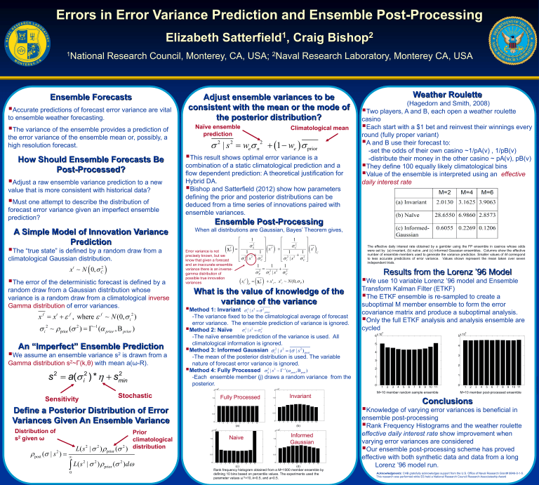
Rank frequency histogram obtained from a M=1000 member ensemble by defining 10 bins based on percentile values. The experiments used the parameter values ω’ 2 =10, k =0.5, and a =0.5.
Weather Roulette
(Hagedorn and Smith, 2008)

Two players, A and B, each open a weather roulette casino

Each start with a $1 bet and reinvest their winnings every round (fully proper variant)

A and B use their forecast to:
-set the odds of their own casino ~1/pA(v) , 1/pB(v)
-distribute their money in the other casino ~ pA(v), pB(v)

They define 100 equally likely climatological bins

Value of the ensemble is interpreted using an
The effective daily interest rate obtained by a gambler using the FP ensemble in casinos whose odds were set by (a) invariant, (b) naïve ,and (c) informed Gaussian ensembles. Columns show the effective number of ensemble members used to generate the variance prediction. Smaller values of M correspond to less accurate predictions of error variance.
Values shown represent the mean taken over seven independent trials.

We use 10 variable Lorenz ’96 model and Ensemble
Transform Kalman Filter (ETKF)

The ETKF ensemble is re-sampled to create a suboptimal M member ensemble to form the error covariance matrix and produce a suboptimal analysis.

Only the full ETKF analysis and analysis ensemble are cycled
6 x 10
4
5 x 10
4
5
4
4
3
3
2
1
2
1
0
1 2 3 4 5 6 7 8 9 10 11
M=10 member random sample ensemble
0
1 2 3 4 5 6 7 8 9 10 11
M=10 member post-processed ensemble
Conclusions

Knowledge of varying error variances is beneficial in ensemble post-processing

Rank Frequency Histograms and the weather roulette
show improvement when varying error variances are considered

Our ensemble post-processing scheme has proved effective with both synthetic data and data from a long
Lorenz ’96 model run.
Acknowledgments: CHB gratefully acknowledges support from the U.S. Office of Naval Research Grant# 9846-0-1-5 .
This research was performed while ES held a National Research Council Research Associateship Award