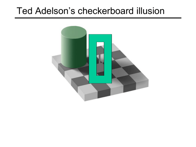
Ted Adelson’s checkerboard illusion
Motion illusion, rotating snakes
Sampling and Reconstruction 2
Slides from Alexei Efros, Fei Fei
Li, Steve Marschner, and others
CS 195g: Computational Photography
James Hays, Brown, Spring 2010
Detailed Recap of Wednesday
Slide credit Fei Fei Li
Slide credit Fei Fei Li
Slide credit Fei Fei Li
Slide credit Fei Fei Li
Image half-sizing
This image is too big to
fit on the screen. How
can we reduce it?
How to generate a halfsized version?
Image sub-sampling
1/8
1/4
Throw away every other row and
column to create a 1/2 size image
- called image sub-sampling
Slide by Steve Seitz
Image sub-sampling
1/2
1/4
(2x zoom)
1/8
(4x zoom)
Aliasing! What do we do?
Slide by Steve Seitz
Gaussian (lowpass) pre-filtering
G 1/8
G 1/4
Gaussian 1/2
Solution: filter the image, then subsample
• Filter size should double for each ½ size reduction. Why?
Slide by Steve Seitz
Subsampling with Gaussian pre-filtering
Gaussian 1/2
G 1/4
G 1/8
Slide by Steve Seitz
Compare with...
1/2
1/4
(2x zoom)
1/8
(4x zoom)
Slide by Steve Seitz
Gaussian (lowpass) pre-filtering
G 1/8
G 1/4
Gaussian 1/2
Solution: filter the image, then subsample
• Filter size should double for each ½ size reduction. Why?
Slide by Steve Seitz
• How can we speed this up?
Image Pyramids
Known as a Gaussian Pyramid [Burt and Adelson, 1983]
• In computer graphics, a mip map [Williams, 1983]
• A precursor to wavelet transform
Slide by Steve Seitz
A bar in the
big images is a
hair on the
zebra’s nose;
in smaller
images, a
stripe; in the
smallest, the
animal’s nose
Figure from David Forsyth
What are they good for?
Improve Search
• Search over translations
– Like project 1
– Classic coarse-to-fine strategy
• Search over scale
– Template matching
– E.g. find a face at different scales
Pre-computation
• Need to access image at different blur levels
• Useful for texture mapping at different resolutions (called
mip-mapping)
Gaussian pyramid construction
filter mask
Repeat
• Filter
• Subsample
Until minimum resolution reached
• can specify desired number of levels (e.g., 3-level pyramid)
The whole pyramid is only 4/3 the size of the original image!
Slide by Steve Seitz
Continuous convolution: warm-up
• Can apply sliding-window average to a continuous function
just as well
– output is continuous
– integration replaces summation
© 2006 Steve Marschner • 45
Continuous convolution
• Sliding average expressed mathematically:
– note difference in normalization (only for box)
• Convolution just adds weights
– weighting is now by a function
– weighted integral is like weighted average
– again bounds are set by support of f(x)
© 2006 Steve Marschner • 46
One more convolution
• Continuous–discrete convolution
– used for reconstruction and resampling
© 2006 Steve Marschner • 47
Reconstruction
© 2006 Steve Marschner • 48
Resampling
• Changing the sample rate
– in images, this is enlarging and reducing
• Creating more samples:
– increasing the sample rate
– “upsampling”
– “enlarging”
• Ending up with fewer samples:
– decreasing the sample rate
– “downsampling”
– “reducing”
© 2006 Steve Marschner • 49
Resampling
• Reconstruction creates a continuous function
– forget its origins, go ahead and sample it
© 2006 Steve Marschner • 50
Cont.–disc. convolution in 2D
• same convolution—just two variables now
– loop over nearby pixels,
average using filter weight
– looks like discrete filter,
but offsets are not integers
and filter is continuous
– remember placement of filter
relative to grid is variable
© 2006 Steve Marschner • 51
A gallery of filters
• Box filter
– Simple and cheap
• Tent filter
– Linear interpolation
• Gaussian filter
– Very smooth antialiasing filter
• B-spline cubic
– Very smooth
© 2006 Steve Marschner • 52
Box filter
© 2006 Steve Marschner • 53
© 2006 Steve Marschner • 54
© 2006 Steve Marschner • 55
© 2006 Steve Marschner • 56
Effects of reconstruction filters
• For some filters, the reconstruction process winds up
implementing a simple algorithm
• Box filter (radius 0.5): nearest neighbor sampling
– box always catches exactly one input point
– it is the input point nearest the output point
– so output[i, j] = input[round(x(i)), round(y(j))]
x(i) computes the position of the output coordinate i on the input
grid
• Tent filter (radius 1): linear interpolation
– tent catches exactly 2 input points
– weights are a and (1 – a)
– result is straight-line interpolation from one point to the next
© 2006 Steve Marschner • 57
Properties of filters
• Degree of continuity
• Impulse response
• Interpolating or no
• Ringing, or overshoot
interpolating filter used for reconstruction
© 2006 Steve Marschner • 58
Ringing, overshoot, ripples
• Overshoot
– caused by
negative filter
values
• Ripples
– constant in,
non-const. out
– ripple free when:
© 2006 Steve Marschner • 59
Yucky details
• What about near the edge?
– the filter window falls off the edge of the image
– need to extrapolate
– methods:
•
•
•
•
•
clip filter (black)
wrap around
copy edge
reflect across edge
vary filter near edge
© 2006 Steve Marschner • 60
Median filters
• A Median Filter operates over a window by selecting the
median intensity in the window.
• What advantage does a median filter have over a mean
filter?
• Is a median filter a kind of convolution?
by Steve
Steve Seitz
©Slide
2006
Marschner • 61
Comparison: salt and pepper noise
by Steve
Steve Seitz
©Slide
2006
Marschner • 62