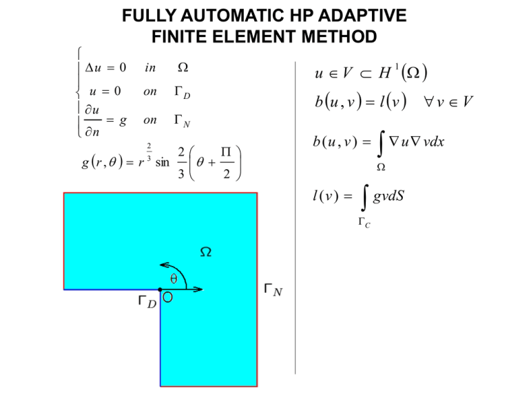
FULLY AUTOMATIC HP ADAPTIVE
FINITE ELEMENT METHOD

 u  0

 u 0
 u
 g

 n
in

on
D
on
N
2
g  r ,    r 3 sin
2
 




3
2 
 
b u , v   l v   v  V
u V  H
b (u , v ) 
1
  u  vdx

l (v ) 
 gvdS
C
FINITE ELEMENT METHOD DISCRETIZATION
The Finite Element Method (FEM)
consists in construction of the finite
dimensional sub-space
V hp  V
We seek the approximate solution
as a linear combination
i
of the V basis functions e hp
hp
21
u hp  V hp
u  u hp 

i 1
i
i
u hp e hp
HP ADAPTATIONi
Goal: increase the number N h p of the basis functions e h p
in order to increase the accuracy of the approximate solution
N hp
u  u hp 

i 1
i
i
u hp e hp
hp adaptation consists in breaking selected finite elements into smaller elements
and increasing polynomial order of approximation on selected finite elements.
FULLY AUTOMATIC HP ADAPTIVE
FINITE ELEMENT METHOD
Coarse mesh
FULLY AUTOMATIC HP ADAPTIVE
FINITE ELEMENT METHOD
Coarse mesh solution
FULLY AUTOMATIC HP ADAPTIVE
FINITE ELEMENT METHOD
Fine mesh
FULLY AUTOMATIC HP ADAPTIVE
FINITE ELEMENT METHOD
Fine mesh solution
FULLY AUTOMATIC HP ADAPTIVE
FINITE ELEMENT METHOD
Optimal mesh is constracted based on comparison of coarse and fine mesh solutions
FULLY AUTOMATIC HP ADAPTIVE
FINITE ELEMENT METHOD
Final mesh delivering solution with 0.001 relative error
FULLY AUTOMATIC HP ADAPTIVE
FINITE ELEMENT METHOD
Zoom 10 X
FULLY AUTOMATIC HP ADAPTIVE
FINITE ELEMENT METHOD
Zoom 100 X
FULLY AUTOMATIC HP ADAPTIVE
FINITE ELEMENT METHOD
Zoom 1000 X
FULLY AUTOMATIC HP ADAPTIVE
FINITE ELEMENT METHOD
Zoom 10000 X
FULLY AUTOMATIC HP ADAPTIVE
FINITE ELEMENT METHOD
Zoom 100000 X
FULLY AUTOMATIC HP ADAPTIVE
FINITE ELEMENT METHOD
Zoom 1000000 X
LOKALNY WYBÓR OPTYMALNEJ STRATEGII ADAPTACJI
Element siatki rzadkiej
Lokalne rozwiązanie na
elemencie siatki rzadkiej
Element siatki gęstej
Lokalne rozwiązanie na
elemencie siatki gęstej
u h, p
uh
2
, p 1
Lokalnie, dla każdego elementu siatki rzadkiej rozważane są różne strategie adaptacji
Dla proponowanych strategii
adaptacji obliczam lokalne
rozwiązanie
poprzez
mechanizm projekcji z
rozwiązania na siatce gęstej
w
???
w
uh
2
, p 1
(mechanizm projekcji)
(dla proponowanych strategii
adaptacji)


Lokalnie, dla każdego elementu siatki rzadkiej,
u h , p 1  u h , p  u h , p 1  w


2
2
wybierana jest taka strategia, która daje nam
max 

największy spadek błędu a jednocześnie najmniejszy

nrdof


przyrost rozmiaru zadania (ilości niewiadomych)


HP ADAPTATION
PROVIDES EXPONENTIAL CONVERGENCE RATE
3D Fichera problem

 u  0

 u 0
 u
 g

 n
2
g  r ,    r 3 sin
w

na
D
na
N

 u  0

 u 0
 u
 g

 n
2
 




3
2 
Laplace equation
w

na
D
na
N
3D Fichera problem
3D Fichera problem
3D Fichera problem
Solution over
the coarse grid
+
=>
+
=>
Solution over
the fine grid
Optimal grid
Relative error estimation (energy norm)
Decisions about optimal h, p or hp refinements
over each coarse grid finite element
3D Fichera problem
3D Fichera problem
3D Fichera problem
Solution over
the coarse grid
+
=>
+
=>
Solution over
the fine grid
Optimal grid
Relative error estimation (energy norm)
Decisions about optimal h, p or hp refinements
over each coarse grid finite element
3D Fichera problem
3D Fichera problem
3D Fichera problem
3D Fichera problem
Results for 3D Fichera problem
Convergence curve for the 3D Fichera problem
Exponential convergence delivered by parallel code
Corresponding fine mesh solution has relative error below 1%
EXEMPLARY BOUNDARY VALUE PROBLEM
HEAT TRANSFER OVER THE L-SHAPE DOMAIN
Strong formulation (Partial Differential Equations)
Find
R    x  u  x   R temperature scalar field, such that
2

where  is the L-shape domain

  u  0 in


on  D
 u 0
 u
 g on  N
boundary     N   D

 n
On  D part of the boundary we define the Dirichlet boundary
condition (zero temperature)
N
On  N part of the boundary we define the Neumanna boundary condition
(heat transfer rate)
2
2
 
g  r ,    r sin   

3
2 
3
STRONG AND WEAK (VARIATIONAL) FORMULATIONS
Strong formulation
Find u temperature scalar field,
of the order of C 2   such that


  u  0 in

on  D
 u 0
 u
 g on  N

 n

2
V   v  L   : 


v
2
 v
2


dx   : tr v   0 on  D 

Weak (variational) formulation
Find u  V
temperature scalar field such that
b u , v   l  v 
b (u , v ) 
v  V
  u  v dx

l (v ) 
 g v dS
N
FINITE ELEMENT METHOD DISCRETIZATION
The Finite Element Method (FEM)
consists in construction of the finite
dimensional sub-space
V hp  V
We seek the approximate solution
as a linear combination
i
of the V basis functions e hp
hp
21
u hp  V hp
u  u hp 

i 1
i
i
u hp e hp
Finite element discretization
 
b u , v   l v   v  V
u V  H
1
u hp  V hp  H
1
 
N hp
u  u hp 

i
i
u hp e hp
i 1
i
u hp , i  1,..., N hp global degrees of freedom
v  e hp , j  1,..., N hp
j
N hp
 
  
b e hp , e hp  l e hp
i
j
j
 j  1,..., N hp
i 1
b (u , v ) 
 k  u  vdx
b ( e hp , e hp )  u hp  k  e hp  e hp dx
i
j
i


l (v ) 

C
gvdS
i
l ( e hp ) 
j

C
j
ge hp dS
j
MESH STRUCTURE
Mesh is based on Euler’s model:
•
finite element is composed of nodes
•
nodes are: vertices, edges, faces, interiors etc.
•
edge consists of 2 vertices
•
face consists of 4 edges
•
interior consists of (i.e. is delimited by) 6 faces
•
…
face
interior
edge
vertex
SHAPE FUNCTIONS
The base of approximation space is composed of global base functions.
These are splines, made of multi-dimensional polynomials. Global base
functions are connected with a node and have supports of one or several
neighbor elements.
(2D example)
global base functions
based on vertices
global base functions
based on edges
global base functions
based on faces
SHAPE FUNCTIONS
Shape function is a restriction of a GBF into a single finite element.
Shape functions are connected with elements,
and are just single multi-dimensional polynomials
 K2 ,1
(2D example)
For example: global edge base function
8
e hp consists of two local
1
 1K, 2
1

K
shape functions:  1K, 2 and  K0 , 2
2 ,1
K2
1
0,2
2
K
 K2 ,1
2 ,0
3
2
K
0,2
3
Typically in 2D we use shape functions of orders up to (9, 9).
Bilinear local shape functions are obligatory for each element.
(not all functions are shown in the pictures for clarity)
2
Relations between 1D 2D and 3D shape functions
Higher dimension shape functions are constructed as tensor products of
several 1D shape functions
1D Hp Finite Element
1D hierarchical shape functions:
2D Hp Finite Element
4 vertices
4 mid-edge nodes
1mid-face nodes
The reference element shape functions are created as tensor products
of 1D hierarchical shape functions
2D Hp Finite Element
Vertex shape functions and second order edge and interior shape functions
1
e hp
3
e hp
5
e hp
2
e hp
4
e hp
8
e hp
7
9
e hp
e hp
14
e hp
16
e hp
17
e hp
2D Hp Finite Element
One bilinear shape function for each of 8 vertices
(order of approximation equal to 1 in each vertex)
2D Hp Finite Element
shape functions for each of 4 mid-edge nodes (various orders of approximation)
2D Hp Finite Element
face bubble shape functions for interior node
Relations between 1D and 2D
Higher dimension shape functions are constructed as tensor products of
several 1D shape functions
3D Fichera problem

 u  0

 u 0
 u
 g

 n
2
g  r ,    r 3 sin
w

na
D
na
N

 u  0

 u 0
 u
 g

 n
2
 




3
2 
Laplace equation
w

na
D
na
N
3D Hp Finite Element
8 vertices
12 mid-edge nodes
6 mid-face nodes
1 middle node
The reference element shape functions are created as tensor products
of 1D hierarchical shape functions
3D Hp Finite Element
One trilinear shape function for each of 8 vertices
(order of approximation equal to 1 in each vertex)
3D Hp Finite Element
shape functions for each of 12 mid-edge nodes (various orders of approximation)
3D Hp Finite Element
face bubble shape functions for each of 6 mid-face nodes
3D Hp Finite Element
bubble shape functions for the middle node
Relations between 1D and 3D
Higher dimension shape functions are constructed as tensor products of
several 1D shape functions
Using templates as an unification tool
Vertices, edges and interiors for different dimensions are created as
instantiation of general Vertex, Edge or Face template
Summary of shape functions dependencies
Higher order shape functions are created as tensor products
of one dimensional shape functions
Summary of shape functions dependencies
Dimension independent code computing shape function value
Using templates as an unification tool
Deriving dimension independent code creating the stiffness matrix and rhs
Using templates as an unification tool
Deriving dimension independent code creating the stiffness matrix and rhs
Using templates as an unification tool
Deriving dimension independent code creating the stiffness matrix and rhs
Using templates as an unification tool
Deriving dimension independent code creating the stiffness matrix and rhs