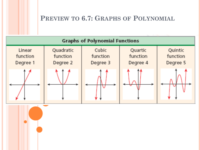
PREVIEW TO 6.7: GRAPHS OF POLYNOMIAL
Example 1: Determining End Behavior of Polynomial Functions
Identify the leading coefficient, degree, and end behavior.
A. Q(x) = –x4 + 6x3 – x + 9
Example 2A: Using Graphs to Analyze Polynomial Functions
Identify whether the function graphed has an odd or even
degree and a positive or negative leading coefficient.
6.9 CURVE FITTING WITH POLYNOMIAL MODELS
Learning Targets:
•Use finite differences to determine the degree of a
polynomial that will fit a given set of data.
•Use technology to find polynomial models for a given
set of data.
Why are we learning this?
The table shows the closing value of a stock index on the first
day of trading for various years.
To create a mathematical model for the data, you will need to
determine what type of function is most appropriate. Then you
can make predictions and make money money money!
WHAT DO WE NEED TO DO TO CREATE
THESE MODELS (FUNCTIONS)?
Analyze the Differences between the y-values!
Example 1A: Using Finite Differences to Determine Degree
Use finite differences to determine the degree of the
polynomial that best describes the data.
x
y
4
–2
6
4.3
8
8.3
10
12
14
10.5 11.4 11.5
The x-values increase by a constant 2. Find the differences of the y-values.
y
–2
4.3
8.3
10.5 11.4 11.5
First differences: 6.3 4
2.2
0.9 0.1 Not constant
Second differences: –2.3 –1.8 –1.3 –0.8
Not constant
Third differences:
0.5 0.5 0.5
Constant
Conclusion:
Once you have determined the degree of the polynomial that best
describes the data, you can use your calculator to create the function.
Example 2: Using Finite Differences to Write a Function
The table below shows the population of a city from 1960
to 2000. Write a polynomial function for the data.
Year
1960
1970
1980
1990
2000
Population
(thousands)
4,267
5,185
6,166
7,830
10,812
Step 1 Find the finite differences of the y-values.
First differences:
918
Second differences:
Third differences:
981
63
1664
683
620
2982
1318
635
Close
Step 2 Use the cubic regression
feature on your calculator.
f(x) ≈ 0.10x3 – 2.84x2 + 109.84x + 4266.79
Often, real-world data can be too irregular for you to use finite differences
or find a polynomial function that fits perfectly. In these situations, you
can use the regression feature of your graphing calculator.
The statistical study of the relationship between variables is called
regression. Correlation is the strength and direction of the linear
relationship between two variables. We can determine a function to
model the data which by using the regression feature on our graphing
calculator. The correlation coefficient r is a measure of how well the
data set is fit by a linear model (the closer r is to 1, the better the model).
The coefficient of determination r^2 shows how well a higher degree
model fits the data (the close r^2 is to 1, the better the fit).
Example 3: Curve Fitting Polynomial Models
The table below shows the opening value of a stock index on the first
day of trading in various years. Use a polynomial model to estimate the
value on the first day of trading in 2000.
Year
1994
1995
1996
1997
1998
1999
Price ($)
683
652
948
1306
863
901
Step 1 Choose possible degrees of the polynomial model by
making a scatter plot of the data in graphing calculator.
Analyze:
Now what?
cubic: R2 ≈ 0.5833 quartic: R2 ≈ 0.8921
The quartic function is more appropriate choice.
Example 3 Continued
Step 2 Write the polynomial model. The data can be modeled by
f(x) = 32.23x4 – 339.13x3 + 1069.59x2 – 858.99x + 693.88
Step 3 Find the value of the model corresponding to 2000.
2000 is 6 years after 1994. Substitute 6 for x in the quartic
model.
f(6) = 32.23(6)4 – 339.13(6)3 + 1069.59(6)2 – 858.99(6) +
693.88
Based on the model, the opening value was about $2563.18 in
2000.