Introduction to Digital Image Processing with MATLAB® Asia Edition
McAndrew‧Wang‧Tseng
Chapter 8:
Image
Restoration
1
© 2010 Cengage Learning
Engineering. All Rights Reserved.
1
8.1 Introduction
• Image restoration concerns the removal or
reduction of degradations that have occurred during
the acquisition of the image
• Some restoration techniques can be performed very
successfully using neighborhood operations, while
others require the use of frequency domain
processes
2
Ch8-p.191
© 2010 Cengage Learning
Engineering. All Rights Reserved.
8.1.1 A Model of Image Degradation
f(x, y) : image
h(x, y) : spatial filter
 Where the symbol ＊ represents convolution
• In practice, the noise n(x, y) must be considered
3
Ch8-p.191
© 2010 Cengage Learning
Engineering. All Rights Reserved.
8.1.1 A Model of Image Degradation
• We can perform the same operations in the frequency
domain, where convolution is replaced by multiplication
• If we knew the values of H and N, we could recover F by
writing the above equation as
this approach may not be practical
4
Ch8-p.192
© 2010 Cengage Learning
Engineering. All Rights Reserved.
8.2 Noise
• Noise—any degradation in the image signal caused by
external disturbance
• These errors will appear on the image output in different
ways depending on the type of disturbance in the signal
• Usually we know what type of errors to expect and the
type of noise on the image; hence, we can choose the
most appropriate method for reducing the effects
5
Ch8-p.192
© 2010 Cengage Learning
Engineering. All Rights Reserved.
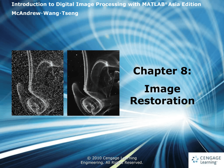
8.2.1 Salt and Pepper Noise
• Also called impulse noise, shot noise, or binary noise,
salt and pepper degradation can be caused by sharp,
sudden disturbances in the image signal
• Its appearance is randomly scattered white or black (or
both) pixels over the image
6
Ch8-p.192
© 2010 Cengage Learning
Engineering. All Rights Reserved.
FIGURE 8.1
>> imshow(t)
7
Ch8-p.193
>> figure, imshow(t_sp)
© 2010 Cengage Learning
Engineering. All Rights Reserved.
8.2.2 Gaussian Noise
• Gaussian noise is an idealized form of white noise,
which is caused by random fluctuations in the signal
• If the image is represented as I, and the Gaussian noise
by N, then we can model a noisy image by simply
adding the two
8
Ch8-p.193
© 2010 Cengage Learning
Engineering. All Rights Reserved.
8.2.3 Speckle Noise
• Speckle noise (or more simply just speckle) can be
modeled by random values multiplied by pixel values
• It is also called multiplicative noise
• imnoise can produce speckle
9
Ch8-p.194
© 2010 Cengage Learning
Engineering. All Rights Reserved.
FIGURE 8.2
10
Ch8-p.194
© 2010 Cengage Learning
Engineering. All Rights Reserved.
8.2.4 Periodic Noise
11
Ch8-p.195
© 2010 Cengage Learning
Engineering. All Rights Reserved.
8.3 Cleaning Salt and Pepper Noise
• Low-Pass Filtering
12
Ch8-p.196
© 2010 Cengage Learning
Engineering. All Rights Reserved.
8.3.2 Median Filtering
13
Ch8-p.197
© 2010 Cengage Learning
Engineering. All Rights Reserved.
FIGURE 8.6
14
Ch8-p.198
© 2010 Cengage Learning
Engineering. All Rights Reserved.
FIGURE 8.7
15
Ch8-p.198
© 2010 Cengage Learning
Engineering. All Rights Reserved.
8.3.3 Rank-Order Filtering
• Median filtering is a special case of a more
general process called rank-order filtering
• A mask as 3×3 cross shape
0
1
0
16
Ch8-p.199
1
1
1
0
1
0
© 2010 Cengage Learning
Engineering. All Rights Reserved.
8.3.4 An Outlier Method
• Applying the median filter can in general be a slow
operation: each pixel requires the sorting of at least nine
values
• Outlier Method
 Choose a threshold value D
 For a given pixel, compare its value p with the mean m of the
values of its eight neighbors
 If |p − m| > D, then classify the pixel as noisy, otherwise not
 If the pixel is noisy, replace its value with m; otherwise leave its
value unchanged
17
Ch8-p.199
© 2010 Cengage Learning
Engineering. All Rights Reserved.
FIGURE 8.8
18
Ch8-p.200
© 2010 Cengage Learning
Engineering. All Rights Reserved.
FIGURE 8.9
19
Ch8-p.201
© 2010 Cengage Learning
Engineering. All Rights Reserved.
8.4 Cleaning Gaussian Noise
• Image Averaging
 suppose we have 100 copies of our image, each with noise
 Because Ni is normally distributed with mean 0, it can be
readily shown that the mean of all the Ni’s will be close to zero
The greater the number of Ni’s; the closer to zero
20
Ch8-p.202
© 2010 Cengage Learning
Engineering. All Rights Reserved.
FIGURE 8.10
21
Ch8-p.203
© 2010 Cengage Learning
Engineering. All Rights Reserved.
8.4.2 Average Filtering
22
Ch8-p.203
© 2010 Cengage Learning
Engineering. All Rights Reserved.
8.4.3 Adaptive Filtering
• Adaptive filters are a class of filters that change
their characteristics according to the values of the
grayscales under the mask
 Minimum mean-square error filter
The noise may not be normally distributed with mean 0
23
Ch8-p.204
© 2010 Cengage Learning
Engineering. All Rights Reserved.
8.4.3 Adaptive Filtering
• Wiener filters (wiener2)
24
Ch8-p.205
© 2010 Cengage Learning
Engineering. All Rights Reserved.
FIGURE 8.12
25
Ch8-p.206
© 2010 Cengage Learning
Engineering. All Rights Reserved.
FIGURE 8.13
26
Ch8-p.206
© 2010 Cengage Learning
Engineering. All Rights Reserved.
8.5 Removal of Periodic Noise
27
Ch8-p.207
© 2010 Cengage Learning
Engineering. All Rights Reserved.
FIGURE 8.15
• BAND REJECT FILTERING
28
Ch8-p.208
© 2010 Cengage Learning
Engineering. All Rights Reserved.
FIGURE 8.16
• NOTCH FILTERING
29
Ch8-p.209
© 2010 Cengage Learning
Engineering. All Rights Reserved.
8.6 Inverse Filtering
30
Ch8-p.210
© 2010 Cengage Learning
Engineering. All Rights Reserved.
FIGURE 8.18
cutoff radius: 60
31
Ch8-p.211
© 2010 Cengage Learning
Engineering. All Rights Reserved.
FIGURE 8.18
cutoff radius: 80
32
Ch8-p.212
cutoff radius: 100
© 2010 Cengage Learning
Engineering. All Rights Reserved.
FIGURE 8.19
d = 0.005
33
Ch8-p.213
© 2010 Cengage Learning
Engineering. All Rights Reserved.
FIGURE 8.19
d = 0.002
34
Ch8-p.213
d = 0.001
© 2010 Cengage Learning
Engineering. All Rights Reserved.
8.6.1 Motion Deblurring
35
Ch8-p.214
© 2010 Cengage Learning
Engineering. All Rights Reserved.
8.6.1 Motion Deblurring
• To deblur the image, we need to divide its
transform by the transform corresponding to
the blur filter
• This means that we first must create a matrix
corresponding to the transform of the blur
36
Ch8-p.215
© 2010 Cengage Learning
Engineering. All Rights Reserved.
FIGURE 8.21
37
Ch8-p.215
© 2010 Cengage Learning
Engineering. All Rights Reserved.
8.7 Wiener Filtering
38
Ch8-p.216
© 2010 Cengage Learning
Engineering. All Rights Reserved.
FIGURE 8.22
K = 0.001
39
Ch8-p.217
© 2010 Cengage Learning
Engineering. All Rights Reserved.
FIGURE 8.22
K = 0.0001
40
Ch8-p.217
K = 0.00001
© 2010 Cengage Learning
Engineering. All Rights Reserved.