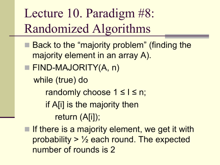
Lecture 10. Paradigm #8:
Randomized Algorithms
 Back to the “majority problem” (finding the
majority element in an array A).
 FIND-MAJORITY(A, n)
while (true) do
randomly choose 1 ≤ I ≤ n;
if A[i] is the majority then
return (A[i]);
 If there is a majority element, we get it with
probability > ½ each round. The expected
number of rounds is 2
Computing ∑s in S Pr[s] s
 Each time a new index of the array is guessed,
we find the majority element with probability p
> 1/2. So the expected number of guesses is
p*1 + (1-p)p*2 + (1-p)2p*3 + ... =
Σi ≥ 1 (1-p)i-1⋅ p ⋅ i = x.
 To evaluate this, multiply x by (1-p) and add y = ∑i ≥ 1
(1-p)i p. We get ∑i ≥ 1 (1-p)i p (i+1), which is just x-p.
Now, using the sum of a geometric series,
Σi ≥ 0 ari = a (1-r∞)/ (1-r)
y evaluates to 1-p. So (1-p)x + (1-p) = x-p. So x = 1/p < 2
Another example: order statistics
 Problem: Given a list of numbers of length n, and an integer i
(with 1 ≤ i ≤ n), determine the i-th smallest member in the list.
 This problem is also called "computing order statistics". Special
cases: computing the minimum corresponds to i = 1, computing
the maximum corresponds to i = n, computing the 2nd largest
corresponds to i = n-1, and computing the median corresponds
to i = ceil(n/2).
 Obviously you could compute the i'th smallest by sorting, but
that takes O(n log n) time, which is not optimal.
 We know how to solve it when i = 1, n-1, n in linear time. We
now give a randomized algorithm to do selection in expected
linear time. By expected (or average) linear time, we mean the
average over all random choices used by the algorithm, and not
depending on the particular input.
Randomized selection
 Remember the PARTITION algorithm for Quicksort in CS240.
 RANDOMIZED-PARTITION chooses a random index j to partition.
 RANDOMIZED-SELECT(A,p,r,i)
/* Find the i'th smallest element from the array A[p..r] */
if p = r then return A[p];
q := RANDOMIZED-PARTITION(A,p,r);
k := q-p+1; /* number of elements in left side of partition */
if i = k then
return A[q] ;
else if i < k
then return RANDOMIZED-SELECT(A,p,q-1,i) ;
else return RANDOMIZED-SELECT(A,q+1,r,i-k);
Expected running time: O(n)
 Expected running time:
T(n) ≤ (1/n)*Σ1 ≤ k ≤ n T(max(k-1,n-k)) + O(n)
 Prove T(n) ≤ cn by induction. Assume it is true for n ≥
3. Now assume it is true for n' < n. Then
 T(n) ≤ ( (1/n)*Σ1 ≤ k ≤ n T(max(k-1,n-k)) ) + O(n)
≤ ((2/n)*Σfloor(n/2) ≤ k ≤ n-1 T(k)) + O(n)
≤ ((2/n)*Σfloor(n/2) ≤ k ≤ n-1 ck) + an (for some a ≥ 1)
= ( (2c/n)*Σfloor(n/2) ≤ k ≤ n-1 k) + an
= ( (2c/n)*(Σ1 ≤ k ≤ n-1 k - Σ1 ≤ k ≤ floor(n/2)-1 k ) + an
≤ (2c/n)* ( n(n-1)/2 - (n/2 - 1)(n/2-2)/2) + an
= (2c/n)*(n2 - n - n2/4 + n + n/2 - 2)/2 + an
= (c/n)*(3n2/4 + n/2 - 2) + an
≤ 3cn/4 + c/2 + an < cn for c large enough.
Example: Matrix multiplication
 Given nxn matrices, A,B,C, test: C=AxB



Trivial O(n3)
Strassen O(nlog7)
Best deterministic alg O(n2.376)
 Consider the following randomized alg:
repeat k times
generate a random nx1 vector x in {-1,1}n ;
if A(Bx) ≠ Cx, then return AB ≠ C;
return AB = C;
Error bound.
Theorem. This algorithm errs with prob ≤ 2-k.
Proof. If C’=AB ≠ C, then for some i, j,
cij ≠ ∑l=1..n ail blj =c’ij
Then C’x ≠ Cx for either xj = 1 or xj = -1. Thus
with probability ½ , one round will tell if AB≠C.
After k rounds, error probability is ≤ 2-k.
Some comments about Randomness
 You might object: in practice, we do not use
truly random numbers, but rather "pseudorandom" numbers. The difference may be
crucial.
 For example, this is one way a
pseudorandom number is generated
Xn+1 = a Xn + c (mod m)
 As von Neumann said in 1951: “Anyone who
considers arithmetical methods of producing
random digits is, of course, in a state of sin."
Which sequence is random?
 If you go to a casino, you flip a coin they provided,
and you get 100 heads in a row. You complain to the
casino: “Your coin is biased, H100 is not a random
sequence!”
 The casino owner would demand: “You give me a
random sequence.”
 You confidently flipped your own coin 100 times and
obtained a sequence S, and tell the casino that you
would trust S to be random.
 But casino can object: the two sequences have the
same probability! Why is S more random than H100
How to define Randomness
 Laplace once said: a sequence is “extraordinary”
(non-random) when it contains regularity.
 Solomonoff, Kolmogorov, Chatin (1960’s): a random
sequence is a sequence that is not (algorithmically)
compressible (by a computer / Turing machine).
Remember, we have used such sequences to obtain
the average case complexity of algorithms.
 In your assignment 2, Problem 2, you have shown:
random sequences exist (in fact, most sequences are
random sequences).