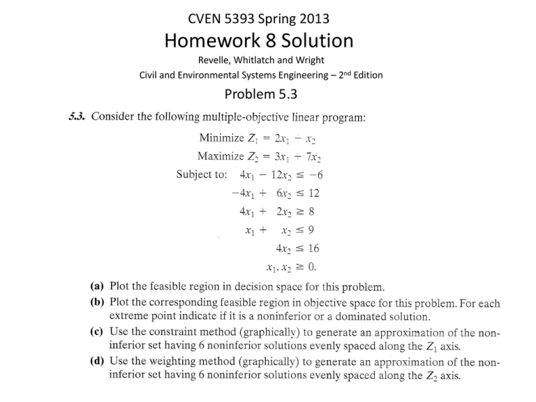
CVEN 5393 Spring 2013
Homework 8 Solution
Revelle, Whitlatch and Wright
Civil and Environmental Systems Engineering – 2nd Edition
Problem 5.3
a) Plot feasible region in decision space
4x1 - 12x2 <= -6
-4x1 + 6x2 <= 12
4x1 + 2x2 >= 8
x1 + x2 <= 9
4x2 <= 16
b) Plot the corresponding feasible
region in objective space. For each
extreme point indicate if it is a
noninferior or dominated solution
Max Z2
Min Z1
Z2
A
B
C
D
E
X1
1.50
0.75
3.00
5.00
6.38
X2
1.00
2.50
4.00
4.00
2.63
Z1
4.00
4.00
10.00
14.00
15.38
Z2
11.50
19.75
37.00
43.00
37.50
dominated
noninferior
noninferior
noninferior
dominated
Z1
C. Use the constraint method (graphically) to generate an approximation of the noninferior set having 6 noninferior solutions evenly spaced along the Z1 axis.
Construct a payoff table. Each row represents the solution of one individual objective function,
and shows the values for the other objects at that point. If alternate optima are detected,
compare the values of other objectives to select the noninferior point. Every point in the payoff
table is a noninferior solution. The table gives the entire range of values each objective can
have on the noninferior set.
Solution
X1
X2
Z1 = 2x1 + x2 min
Z2 = 3x1 + 7x2 max
Z1 Optima
1.5
.75
1.0
2.5
4.0
4.0
11.50
19.75
A
B
Z2 Optima
5.0
4.0
14.0
43.00
D
Need 6 noninferior solutions evenly spaced along the Z1 axis
Max is 14; Min is 4.0 Other 4 points are 6, 8, 10, 12
Create constrained problem by selecting one of the objectives to optimize and moving the other(s) into
the constraint set with the addition of a right hand side coefficient for each. 4 additional constraints to
add to the problem, one at a time and find optimal solution for Z2:
2X1 + X2 <= 6
2X1 + X2 <= 8
2X1 + X2 <= 10
2X1 + X2 <= 12
-
-
X2
Add each additional
constraint to the set and find the optimal solution for the
remaining objective.
Each solution- is a noninferior solution of the multiobjective problem.
Decision Space
4x1 - 12x2 <= -6
Series1
10
-4x1 + 6x2 <= 12
- 2x + x <= 12
Series2
1
2
4x1 + 2x2 >= 8
9
Series3
x1 + x2 <= 9
2x1 + x2 <= 10
2x1 + x2 <= 14
8
Series4
4x2 <= 16
Series5
2x1 + x2 <= 6
7
2x1 + x2 <= 8
New constraint set:
6
2X1 + X2 <= 6
2X1 + X2 <= 8
5
- - 2X1 + X2 <= 10
2x1 + x2 <= 6
- - 2X1 + X2 <= 12
4
- - Noninferior Solutions
3
- - X1
X2
Z1
Z2
2
0.75
2.50
4.00
19.75
1.50
3.00
6.00
25.50
Max
3X
+
7X
1
2
2.25
3.50
8.00
31.25
1
3.00
4.00
10.00
37.00
4.00
4.00
12.00
40.00
0
5.00
4.00
14.00
43.00
0
4
6
8
10
12
- 2
X1
-
c) The selection of the Z1 points gave
the same solution for the pareto
front as we got in a) and b). If we had
not used as many Z1 points we may
have gotten some approximation
errors.
Max Z2
Min Z1
Z2
A
B
C
D
E
X1
1.50
0.75
3.00
5.00
6.38
X1
0.75
1.50
2.25
3.00
4.00
5.00
X2
1.00
2.50
4.00
4.00
2.63
X2
2.50
3.00
3.50
4.00
4.00
4.00
Z1
4.00
4.00
10.00
14.00
15.38
Z1
4.00
6.00
8.00
10.00
12.00
14.00
Z2
11.50
19.75
37.00
43.00
37.50
dominated
noninferior
noninferior
noninferior
dominated
Z2
19.75
25.50
31.25
37.00
40.00
43.00
Z1
d.) Use the weighting method (graphically) to generate an approximiation of the noninferior set having 6 noninferior solutions evenly spaced along the Z2 axis.
What is range of Z2 point?
We know this from the payoff table. Z2 ranges from 19.75 to 43.0.
Six evenly space values are: Z2 = 19.75; 24.40; 29.05; 33.70; 38.35; 43.0
To solve: use the weighting method to identify noninferior points in objective space.
Then interpolate between these to find the value of noninferior points at the
designated Z2 values. Note that since Z1 is a minimization objective and Z2 is a max
objective, we must make Z1 also a max objective by taking the negative of it.
We arbitrarily select a set of weights and compute the Grand Objective:
grad
ient
w1
w2
w1*(-)Z1 + w2*Z2
Grand objective
1
1.0
0
1.0 * (-2x1 – x2) + 0*(3x1+7x2)
Max -2x1 – x2
2
0.8
0.2
0.8 * (-2x1 – x2) + 0.2*(3x1+7x2)
Max -x1 + 0.6x2
3
0.6
0.4
0.6 * (-2x1 – x2) + 0.4*(3x1+7x2)
Max 2.2x2
4
0.4
0.6
0.4 * (-2x1 – x2) + 0.6*(3x1+7x2)
Max x1 + 3.8x2
5
0.2
0.8
0.2 * (-2x1 – x2) + 0.8*(3x1+7x2)
Max 2.0x1 + 5.4x2
6
0
1.0
0 * (-2x1 – x2) + 1.0*(3x1+7x2)
Max 3x1 + 7x2
d) Solve single grand objectives
4x1 - 12x2 <= -6
-4x1 + 6x2 <= 12
4x1 + 2x2 >= 8
x1 + x2 <= 9
4x2 <= 16
Gr Objective
1 -2x1 – x2
2 -x1 + 0.6x2
3 2.2x2
4 x1 + 3.8x2
5 2.0x1 + 5.4x2
6 3x1 + 7x2
Solution
A,B
B
C,D
D
D
D
x1 x2
Z1
Z2
0.75 2.5 4.0 19.75
0.75 2.5 4.0 19.75
3.0
5.0
5.0
5.0
5.0
4.0 10.0 37.0
4.0 14.0 43.0
4.0 14.0 43.0
4.0 14.0 43.0
4.0 14.0 43.0
b) Use linear interpolation to find the
noninferior points at Z2 = 19.75;
24.40; 29.05; 33.70; 38.35; 43.0
50
45
14, 43
40
10.9, 38.35
10, 37
Z2
19.75
24.40
29.05
33.70
38.35
43.00
Z1
4.0
5.62
7.64
8.85
10.9
14.0
35
8.85, 33.7
Z2
30
7.64, 29.05
25
5.62, 24.4
20
Series1
4, 19.75
15
10
5
0
0
5
10
Z1
15
Things to keep in mind
The “classical” methods of solving multi-objective optimization problems are based
on creating a set of single objective optimization problems, each of which identifies a
non-inferior solution. The set forms a pareto front or surface (if more than 2-d). Other
solutions can be inferred by interpolation if the variables are continuous.
If you have a plot of extreme points in objective space, you can identify the
noninferior extreme points by the relative values of the objectives or by the “corner”
rule. The NE corner rule depends on sign of objectives
The payoff table identifies the range of values that each objective can have.