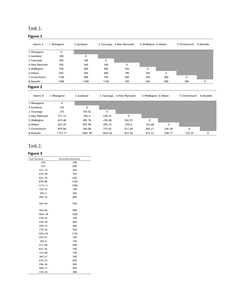
Task 1:
Figure 1
Matrix A
1.Whangarei
1.Whangarei
2.Auckland
3.Tauranga
4.New Plymouth
5.Wellington 6.Nelson
7.Christchurch
8.Dunedin
0
2.Auckland
100
0
3.Tauranga
200
100
0
4.New Plymouth
420
360
140
0
5.Wellington
750
600
460
350
0
6.Nelson
620
550
400
190
150
0
7.Christchurch
1100
900
750
500
350
280
0
8.Dunedin
1500
1200
1150
750
650
500
380
1.Whangarei
2.Auckland
0
Figure 2
Matrix B
1.Whangarei
3.Tauranga
4.New Plymouth
5.Wellington 6.Nelson
7.Christchurch
0
2.Auckland
162
0
3.Tauranga
272
154.52
0
4.New Plymouth
371.14
252.4
238.43
0
5.Wellington
619.48
492.76
418.28
252.91
0
6.Nelson
623.76
507.99
470.15
255.6
124.68
0
7.Christchurch
879.86
764.06
715.42
511.69
305.21
256.36
0
8.Dunedin
1173.11
1063.78
1024.42
812.36
615.23
558.17
310.34
Task 2:
Figure 3
True Distance
8.Dunedin
Estimated Distance
162
100
272
200
371.14
420
619.48
750
623.76
620
879.86
1100
1173.11
1500
154.52
100
252.4
360
492.76
600
507.99
550
764.06
900
1063.78
1200
238.43
140
418.28
460
470.15
400
715.42
750
1024.42
1150
252.91
350
255.6
190
511.69
500
812.36
750
124.68
150
305.21
350
615.23
650
256.36
280
558.17
500
310.34
380
0
Figure 4
Scatter Plot of Estimated Distance vs True Distance
Figure 5
Regression Table for Estimated Distance vs True Distance
SUMMARY OUTPUT
Regression Statistics
Multiple R
0.98
R Square
0.9541
Adjusted R Square
0.95
Standard Error
78.67
Observations
28
Coefficients
Standard Error
t Stat
P-value
Lower 95%
Upper 95%
Lower 95.0%
Upper 95.0%
Intercept
-63.82
30.31
-2.11
0.05
-126.13
-1.51
-126.13
-1.51
True Distance
1.2098
0.05
23.24
6.43E-19
1.10
1.32
1.10
1.32
ANOVA
df
MS
F
1
3342078.96
3342078.96
539.98
Residual
26
160921.04
6189.27
Total
27
3503000
Regression
SS
Significance F
6.4E-19
Task 3:
Multiple regression analysis was used to test the accuracy between my estimated distances
between pairs of cities in New Zealand, and its true distances. My estimates were captured by
a straight line, maintaining a close estimation to the true distances. A small degree of freedom
indicates a strong correlation between our two variables, suggesting that my mentally mapped
estimated distances were close in accuracy. The Multiple R value of 0.98 indicates a very
strong linear relationship between the two variables. A significant p value indicates statistical
significance of the regression model.
The slope of the best fitting line is y =1.2098x - 63.82. The negative coefficient value -63.82
reveals that as the estimated distance increases, the true distance decreases. There is a
significant decrease between the values of the true distances with the estimated distances, t(1)
= -2.11. This suggests that I tended to overestimate the value of linear distances between city
pairs when mental mapping; this is also evident in Figure 3. The results of the regression
indicate that 95.41% of the variance in the true distances can be explained by the estimated
distances (R2 =0.9541, F(1, 539.98) = 6.43, p = 0.05).