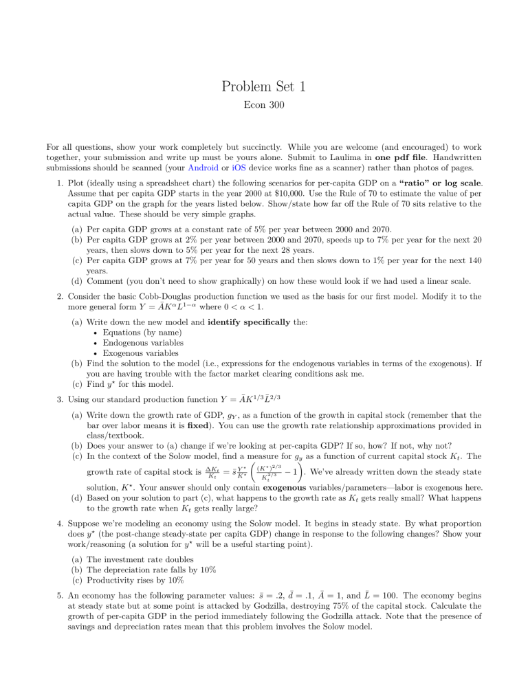
Problem Set 1
Econ 300
For all questions, show your work completely but succinctly. While you are welcome (and encouraged) to work
together, your submission and write up must be yours alone. Submit to Laulima in one pdf file. Handwritten
submissions should be scanned (your Android or iOS device works fine as a scanner) rather than photos of pages.
1. Plot (ideally using a spreadsheet chart) the following scenarios for per-capita GDP on a “ratio” or log scale.
Assume that per capita GDP starts in the year 2000 at $10,000. Use the Rule of 70 to estimate the value of per
capita GDP on the graph for the years listed below. Show/state how far off the Rule of 70 sits relative to the
actual value. These should be very simple graphs.
(a) Per capita GDP grows at a constant rate of 5% per year between 2000 and 2070.
(b) Per capita GDP grows at 2% per year between 2000 and 2070, speeds up to 7% per year for the next 20
years, then slows down to 5% per year for the next 28 years.
(c) Per capita GDP grows at 7% per year for 50 years and then slows down to 1% per year for the next 140
years.
(d) Comment (you don’t need to show graphically) on how these would look if we had used a linear scale.
2. Consider the basic Cobb-Douglas production function we used as the basis for our first model. Modify it to the
more general form Y = ĀK α L1−α where 0 < α < 1.
(a) Write down the new model and identify specifically the:
• Equations (by name)
• Endogenous variables
• Exogenous variables
(b) Find the solution to the model (i.e., expressions for the endogenous variables in terms of the exogenous). If
you are having trouble with the factor market clearing conditions ask me.
(c) Find y ⋆ for this model.
3. Using our standard production function Y = ĀK 1/3 L̄2/3
(a) Write down the growth rate of GDP, gY , as a function of the growth in capital stock (remember that the
bar over labor means it is fixed). You can use the growth rate relationship approximations provided in
class/textbook.
(b) Does your answer to (a) change if we’re looking at per-capita GDP? If so, how? If not, why not?
for g
(c) In the context of the Solow model, find a measure
y as a function of current capital stock Kt . The
growth rate of capital stock is
∆Kt
Kt
⋆
Y
= s̄ K
⋆
(K ⋆ )2/3
2/3
Kt
− 1 . We’ve already written down the steady state
solution, K ⋆ . Your answer should only contain exogenous variables/parameters—labor is exogenous here.
(d) Based on your solution to part (c), what happens to the growth rate as Kt gets really small? What happens
to the growth rate when Kt gets really large?
4. Suppose we’re modeling an economy using the Solow model. It begins in steady state. By what proportion
does y ⋆ (the post-change steady-state per capita GDP) change in response to the following changes? Show your
work/reasoning (a solution for y ⋆ will be a useful starting point).
(a) The investment rate doubles
(b) The depreciation rate falls by 10%
(c) Productivity rises by 10%
5. An economy has the following parameter values: s̄ = .2, d¯ = .1, Ā = 1, and L̄ = 100. The economy begins
at steady state but at some point is attacked by Godzilla, destroying 75% of the capital stock. Calculate the
growth of per-capita GDP in the period immediately following the Godzilla attack. Note that the presence of
savings and depreciation rates mean that this problem involves the Solow model.