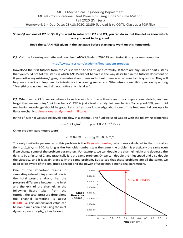
METU Mechanical Engineering Department
ME 485 Computational Fluid Dynamics using Finite Volume Method
Fall 2020 (Dr. Sert)
Homework 1 – Due Date: 28/10/2020, 23:59 (Upload it to ODTU Class as a PDF file)
Solve Q1 and one of Q2 or Q3. If you want to solve both Q2 and Q3, you can do so, but then let us know which
one you want to be graded.
Read the WARNINGS given in the last page before starting to work on this homework.
Q1. Visit the following web site and download ANSYS Student 2020 R2 and install it on your own computer.
http://www.ansys.com/academic/free-student-products
Download the first tutorial from the course web site and study it carefully. If there are any unclear parts, steps
that you could not follow, steps in which ANSYS did not behave in the way described in the tutorial document or
if you notice any mistakes/typos, take notes about them and submit them as an answer to this question. They will
help me correct and improve the tutorial for the coming semesters. Otherwise answer this question by writing
“Everything was clear and I did not notice any mistakes”.
Q2. When we do CFD, we sometimes focus too much on the software and the computational details, and we
forget that we are doing “fluid mechanics”. CFD is just a tool to study fluid mechanics. To do good CFD, your fluid
mechanics knowledge should be good. Let’s refresh our knowledge about one of the fundamental concepts in
fluids mechanics; dimensional analysis and similitude.
In the 1st tutorial we studied developing flow in a channel. The fluid we used was air with the following properties
𝜌 = 1.2 kg/m3 ,
𝜇 = 1.8 × 10−5 Pa ⋅ s
Other problem parameters were
𝐻 = 0.1 m
,
𝑈𝑖𝑛 = 0.015 m/s
The only similarity parameter in this problem is the Reynolds number, which was calculated in the tutorial as
𝑅𝑒 = 𝜌𝑈𝑖𝑛 𝐻/𝜇 = 100. As long as the Reynolds number stays the same, the problem is practically the same even
if we change some of the problem parameters. For example, we can double the channel height and decrease the
density by a factor of 2, and practically it is the same problem. Or we can double the inlet speed and also double
the viscosity, and it is again practically the same problem. But to see that these problems are all the same, we
need to be aware of the similitude concept and the power of using non-dimensional parameters.
One of the important results in
simulating a developing channel flow is
the total pressure drop., i.e. the
pressure difference between the inlet
and the exit of the channel. In the
following figure taken from the
tutorial, the total pressure drop along
the channel centerline is about
0.0004 Pa. This dimensional value can
be non-dimensionalized using the inlet
2
dynamic pressure 𝜌𝑈𝑖𝑛
/2 as follows
Δ𝑝 ≈ 0.0004 Pa
1
Δ𝑝∗ =
Δ𝑝
=
2
𝜌𝑈𝑖𝑛
/2
0.0004 Pa
= 2.96
kg
m 2
(1.2 3 ) (0.015 s ) /2
m
When we say “As long as the Reynolds number does not change, the problem remains practically the same even
if the problem parameters change”, we mean that these kind of non-dimensional parameters are expected not to
change. Let’s check whether this is really the case or not by solving the following problems.
a) Solve the tutorial problem using water with the following properties defined in Fluent’s database
𝜌𝑤𝑎𝑡𝑒𝑟 = 998.2 kg/m3



,
𝜇𝑤𝑎𝑡𝑒𝑟 = 1.0034 × 10−3 Pa ⋅ s
Using 𝐻 = 0.1 m, determine 𝑈𝑖𝑛 that will give 𝑅𝑒 = 100.
Provide the graph showing the pressure variation along the channel centerline. Calculate the
dimensional Δ𝑝.
Calculate the non-dimensional Δ𝑝∗ and check whether it matches with the one calculated above.
b) This time use glycerin (a very viscous liquid) with the following properties defined in Fluent’s database
𝜌𝑔𝑙𝑦𝑐𝑒𝑟𝑖𝑛 = 1259.9 kg/m3



,
𝜇𝑔𝑙𝑦𝑐𝑒𝑟𝑖𝑛 = 0.799 Pa ⋅ s
Using 𝐻 = 0.1 m, determine 𝑈𝑖𝑛 that will give 𝑅𝑒 = 100.
Provide the graph showing the pressure variation along the channel centerline. Calculate the
dimensional Δ𝑝.
Calculate the non-dimensional Δ𝑝∗ and check whether it matches with the one calculated above.
c) Comment of your findings. What is the advantage of using non-dimensional parameters instead of
dimensional ones?
d) Discuss what change (if any) will happen in this similitude discussion and the related findings, if we also play
with the channel height? For example, if we use air, decrease the channel height by a factor of 2 and keep
the Reynolds number the same by increasing the inlet speed by a factor of 2.
e) I claim that “Similitude and dimensional analysis are more critical for experimental studies compared to
CFD simulations”. Do you agree? Why, why not? Discuss.
Hint: To perform new Fluent solutions, open the ANSYS Workbench file that you already created for the tutorial,
save it with a different name. Double click on the Solution cell (not the Setup cell) to start Fluent. This way all your
previous work including the plots you generated earlier will be accessible. All you need to do is change the fluid
properties, change the inlet speed, initialize the solution, run and post-process.
Hint: To select a fluid from Fluent’s database, start like creating a new fluid, press the Fluent Database button and
select the desired fluid. When there are multiple fluids defined in an analysis, you need to make sure that the
correct one is used in the solution. To do this, double click on fff_channel under Cell Zone Conditions and select
the fluid you want to use. After this, you can delete the unnecessary fluids if you want. If you are not allowed to
delete an unnecessary fluid, it means it is still in use and you are probably doing something wrong.
Hint: You are advised to initialize the solution before performing a new run.
Hint: When you plot something in Fluent and all you see is the residual figure, it means that you are looking at the
wrong plot tab. Just make the other plot tab in the graph window visible to see the new figure.
2
Q4. Let’s modify the geometry and physics of the tutorial problem as follows. Now it is a heat transfer problem
with cold and hot fluid streams mix.
𝐿=1m
𝑈𝑙𝑒𝑓𝑡 = 0.015 m/s
𝑇𝑙𝑒𝑓𝑡 = 283 K
𝑝=0
𝐻 = 0.1 m
0.2 m
0.03 m
0.1 m
All walls are insulated
𝑈𝑏𝑜𝑡𝑡𝑜𝑚
𝑇𝑏𝑜𝑡𝑡𝑜𝑚 = 363 K
Main channel dimensions are the same as before. But now there is a second smaller channel attached to it. Cold
fluid at 10 oC = 283 K enters from the left inlet at 0.015 m/s speed. Hot fluid at 90 oC = 363 K enters from the
bottom inlet at a speed that will vary. Duct walls are assumed to be isolated, i.e. there is no heat transfer from
them to the surrounding.
Working fluid is air with the following properties taken at an average temperature of 50 oC.
𝜌 = 1.09
kg
m3
,
𝜇 = 1.96 × 10−5 Pa ⋅ s
, 𝑐𝑝 = 1006.3
J
kgK
,
𝑘 = 0.0282
W
mK
This channel is used to heat up the cold main fluid by mixing it with the hot one. But we do not want the maximum
temperature at the outlet exceed 65 oC = 338 K. You are asked to determine the maximum allowable bottom inlet
speed so that this condition is satisfied.
Perform CFD solutions for various bottom inlet speeds such as 0.015 m/s, 0.03 m/s, 0.045 m/s, etc. (you can select
these speeds in any way you want) and for each run provide the following results






Used bottom inlet speed
Pathlines (starting from both inlets)
Temperature field contour
Variation of temperature at the exit of the channel (as an XY plot in Fluent)
Maximum temperature at the exit
One paragraph discussion of the results/plots. You can do comparisons of different cases.
After performing enough number of runs with different bottom inlet speeds, plot the variation of maximum exit
temperature vs. bottom inlet speed. Based on this plot, determine the maximum allowed bottom inlet speed so
that the maximum exit temperature does not exceed 65 oC.
Hints:





Do not forget to set the viscous model to laminar.
Activate the energy solver to get the temperature field.
To set an inlet temperature, use the Thermal tab of the inlet boundary condition window.
The default thermal boundary condition at the walls is “zero flux”, i.e. insulated.
You do not need to create a new ANSYS Workbench project for each solution. After setting up, solving,
and post-processing one case, you can change the bottom inlet speed, initialize the solution, solve and
post-process the next case, and continue like this.
3
WARNINGS












THIS IS AN INDIVIDUAL ASSIGNMENT. EVERYTHING IN YOUR REPORT SHOULD BE THE RESULT OF YOUR
OWN WORK.
SUBMIT A SINGLE PDF FILE AS YOUR HOMEWORK REPORT. DO NOT SUBMIT ANY ANSYS FILES.
NAME YOUR PDF FILE AS “YOUR NAME – Student ID.PDF”.
PAY ATTENTION TO THE FORMAT OF YOUR REPORT. MAKE SURE THAT IT IS IN THE BEST POSSIBLE
FORM.
DO NOT USE APPENDICES IN YOUR REPORT.
A REPORT THAT IS FULL OF FIGURES WITH TOO LITTLE OR NO EXPLANATION/DISCUSSION WILL NOT
GET A GOOD GRADE. YOU NEED TO DO COMPUTATIONAL FLUID DYNAMICS, NOT COLORFUL FLUID
DYNAMICS.
MAKE SURE THAT ALL THE FIGURES HAVE A FIGURE NUMBER AND CAPTION.
WHEN YOU TAKE SCREENSHOTS CROP THEM PROPERLY AND ONLY PROVIDE THE NECESSARY PARTS,
NOT THE WHOLE PROGRAM WINDOW OR THE WHOLE SCREEN.
YOU ARE ADVISED TO CHANGE THE BACKGROUND COLOR OF THE GRAPHICS WINDOW OF FLUENT TO
WHITE TO HAVE BETTER LOOKING PLOTS.
PROVIDE FIGURES THAT ARE LARGE ENOUGH TO SEE THE DETAILS, BUT NOT LARGER. TRY TO PUT
MULTIPLE FIGURES ON ONE PAGE WHENEVER POSSIBLE. DO NOT USE UNNECESSARILY LARGE FONTS
OR MARGINS.
IF DETAILS ARE HARD TO SEE IN A FIGURE, PROVIDE A CLOSE UP VIEW.
IF NECESSARY, CHANGE THE FORMAT (LINE STYLES, COLORS, AXES NAMES, AXES NUMER FORMAT,
ETC.) OF THE FIGURES FLUENT GENERATES TO GET BETTER LOOKING FIGURES.
4