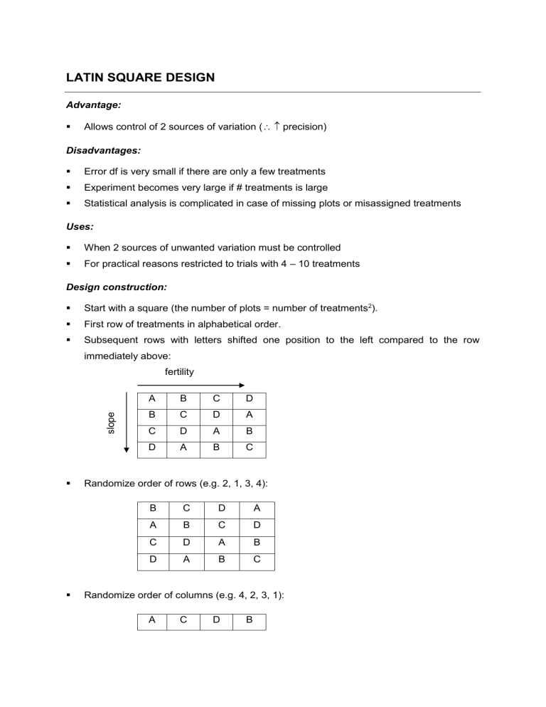
LATIN SQUARE DESIGN
Advantage:

Allows control of 2 sources of variation (  precision)
Disadvantages:

Error df is very small if there are only a few treatments

Experiment becomes very large if # treatments is large

Statistical analysis is complicated in case of missing plots or misassigned treatments
Uses:

When 2 sources of unwanted variation must be controlled

For practical reasons restricted to trials with 4 – 10 treatments
Design construction:

Start with a square (the number of plots = number of treatments2).

First row of treatments in alphabetical order.

Subsequent rows with letters shifted one position to the left compared to the row
immediately above:
slope
fertility


A
B
C
D
B
C
D
A
C
D
A
B
D
A
B
C
Randomize order of rows (e.g. 2, 1, 3, 4):
B
C
D
A
A
B
C
D
C
D
A
B
D
A
B
C
Randomize order of columns (e.g. 4, 2, 3, 1):
A
C
D
B
D
B
C
A
B
D
A
C
C
A
B
D
Analysis:
The procedure of analysis is similar to the randomized and randomized block designs.
Row x column table of observations and totals for Latin square design
Column
Row
1
2
3
4
Sum
1
y11
y12
y13
y14
R1
2
y21
y22
y23
y24
R2
3
y31
y32
y33
y34
R3
4
y41
y42
y43
y44
R4
Sum
C1
C2
C3
C4
G
Treatment totals and means for Latin square design
Treatments
Rep.
1
2
3
4
1
y11
y12
y13
y14
2
y21
y22
y23
y24
3
y31
y32
y33
y34
4
y41
y42
y43
y44
Sum
Sum
T1
T2
T3
T4
G
Mean
y1
y2
y3
y4
y
ANOVA-table for Latin square design (n = p2)
Source
df
SS
MS
F
Treatment
p–1
SST
MST
FT
Row
p–1
SSR
MSR
FR
Column
p–1
SSC
MSC
FC
Error
(p – 1)(p – 2)
SSE
MSE
Total
n–1
SSTot
CF = G2/n (correction factor)
MST = SST/dfT
FT = MST/MSE
SSTot = [ all (observations)2] – CF
MSR = SSR/dfR
FR = MSR/MSE
SST = [1/r x  all(T2)] – CF
MSC = SSC/dfC
FC = MSC/MSE
SSR = [1/p x  all(R2)] – CF
MSE = SSE/dfE
SSC = [1/p x  all(C2)] – CF
SSE = SSTot – SST – SSR – SSC
FACTORIAL EXPERIMENTS
Interactions
The traditional approach is to look at only one factor in an experiment. But a researcher can
also evaluate the influence of more factors in a single experiment, e.g. cultivar (C) and nitrogen
level (N):
C1
C1
C2
C2
Yield
Yield
C3
C3
A
0
20
40
60
80
B
0
20
40
60
80
Nitrogen level (kg/ha)
Main effects: Factors act independently of each other, e.g. every cultivar reacts in the same
way towards the increasing N-level (A).
Interaction: The effects of two or more factors are not independent from each other, e.g.
different cultivars react differently towards increasing N fertilization (B).
Factorial experiments
Interactions are very common. If an experiment is planned to enable measurement and testing
of interactions between different factors, we call it a factorial experiment. Note, this is not an
experimental design, it only describes the nature of the treatments!
Advantages:

Saves time and materials for two reasons:
-
Main effects are all that are required to describe the results.
-
Hidden replication.
Disadvantages:

As the number of factors increases, there is a great increase in the number of treatments.

Large factorials are difficult to interpret, especially if interactions are present.
Uses:

Exploratory experiments – to determine which factors are important.

To study relationships among a number of factors.

Trails designed to make recommendations over a wide range of conditions (conditions
included as factors)
Layout:

Choose an experimental design appropriate for the site of the trial.

The treatments will look a bit different, as there will be more than one factor.
Analysis:

Follows the same pattern as the single factor experiments already discussed.
Two-factor experiments
Say an experiment is performed with two factors, A and B. A at 3 levels and B at 2 levels and
a randomized block design with 4 blocks is used:
Number of plots = A x B x blocks = 3 x 2 x 4 = 24 plots
Treatments = 3 x 2 = 6 different treatment combinations
A1B1
A1B2
A2B1
A2B2
A3B1
A3B2
Design construction:
I
II
III
IV
A2B1
A3B2
A2B2
A1B1
A3B1
A1B1
A1B2
A3B1
A1B1
A3B1
A1B2
A3B2
A2B1
A1B2
A3B2
A2B2
A1B2
A2B2
A3B1
A2B1
A3B2
A2B2
A1B1
A2B1
Analysis:
Table of treatment observations, means and totals for a two-factor experiment
(RBD)
Factors
A1
A2
A3
Block
B1
B2
B1
B2
B1
B2
Sum
1
y11
y12
y13
y14
y15
y16
R1
2
y21
y22
y23
y24
y25
y26
R2
3
y31
y32
y33
y34
y35
y36
R3
4
y41
y42
y43
y44
y45
y46
R4
Sum
T11
T12
T21
T22
T31
T32
G
Mean
y11
y12
y21
y 22
y31
y32
y
Two-way table of factor A and B totals
Factor B
Factor A
1
2
Sum
1
T11
T12
A1
2
T21
T22
A2
3
T31
T32
A3
Sum
B1
B2
G
ANOVA for a 2-factor factorial experiment (RBD)
Source
df
SS
MS
F
A
a–1
SSA
MSA
FA
B
b–1
SSB
MSB
FB
AB
(a – 1)(b – 1)
SSAB
MSAB
FAB
Block
r–1
SSR
MSR
FR
Error
(r – 1)(ab – 1)
SSE
MSE
Total
rab - 1
SSTot
CF = G2/n (Correction Factor)
MSX = SSX/dfX
SSTot = [ all (observations)2] – CF
FA = MSA/MSE
SSA = [1/rb x  all(A2)] – CF
FB = MSB/MSE
SSB = [1/ra x  all(B2)] – CF
FAB = MSAB/MSE
SSAB = [1/r x  all(T2)] – CF – SSA – SSB
FR = MSR/MSE
SSR = [1/p x  all(R2)] – CF
SSE = SSTot – SSA – SSB – SSAB – SSR
Important: As a general rule we do not look at the main effecs if the interaction is significant,
in other words, you should only report on the interaction. Only if the interaction is not significant
one should consider the significance of main effects.
THREE-FACTOR EXPERIMENTS
The same procedures are followed as for two-factor experiments, but more complicated
interactions are involved.
Effects that should be considered:

3 main effects (A; B; C)

3 first order interactions (AxB; AxC; BxC)

1 second order interaction (AxBxC)

Block (randomized block design) / row and column (Latin square design)
Example:
Say factor A (2 levels), factor B (2 levels), and factor C (3 levels) are investigated. The
experiment is planned according to the completely randomized design with 3 replications.
Number of plots = 2 x 2 x 3 x 3 = 36 plots
Treatments = 2 x 2 x 3 = 12 combinations
A1B1C1
A1B2C1
A2B1C1
A2B2C1
A1B1C2
A1B2C2
A2B1C2
A2B2C2
A1B1C3
A1B2C3
A2B1C3
A2B2C3
Design construction:
(Completely randomised design)
A1B1C3
A2B1C3
A2B1C2
A1B1C1
A2B1C1
A1B1C2
A1B2C3
A2B2C2
A1B1C2
A2B1C3
A1B2C2
A2B2C3
A2B1C1
A1B1C1
A1B2C1
A1B1C3
A2B2C2
A2B2C1
A2B2C1
A2B1C2
A2B2C3
A1B2C3
A2B1C2
A1B2C2
A1B2C1
A2B2C1
A1B2C2
A2B1C1
A1B1C1
A2B1C3
A2B2C3
A1B1C3
A2B2C2
A1B1C2
A1B2C3
A1B2C1
Table of observations, totals and means for treatments (CRD)
A1
A2
B1
B2
B1
B2
C2
C3
C1
C2
C3
C1
C2
C3
C1
C2
C3
y1111
y1112
y1113
y1121
y1122
y1123
y1211
y1212
y1213
y1221
y1222
y1223
y2111
y2112
y2113
y2121
y2122
y2123
y2211
y2212
y2213
y2221
y2222
y2223
y3111
y3112
y3113
y3121
y3122
y3123
y3211
y3212
y3213
y3221
y3222
y3223
T111
T112
T113
T121
T122
T123
T211
T212
T213
T221
T222
T223
G
y111
y112
y113
y121
y122
y123
y 211
y212
y213
y 221
y222
y223
y
Sum
C1
Three-way table of factor totals
C
A
B
1
2
3
Sum
1
1
T111
T112
T113
T11.
2
T121
T122
T123
T12.
Sum
T1.1
T1.2
T1.3
A1
1
T211
T212
T213
T21.
2
T221
T222
T223
T22.
Sum
T2.1
T2.2
T2.3
A2
C1
C2
C3
G
2
Sum
Two-way table of AC totals
Two-way table of AB totals
Factor C
Factor B
Factor A
1
2
Sum
Factor A
1
2
3
Sum
1
T11.
T12.
A1
1
T1.1
T1.2
T1.3
A1
2
T21.
T22.
A2
2
T2.1
T2.2
T2.3
A2
Sum
B1
B2
G
Sum
C1
C2
C3
G
Two-way table of BC totals
Factor C
Factor B
1
2
3
Sum
1
T.11
T.12
T.13
B1
2
T.21
T.22
T.23
B2
Sum
C1
C2
C3
G
ANOVA for 3-factor factorial experiment (CRD)
Source
df
SS
MS
F
A
a–1
SSA
MSA
FA
B
b–1
SSB
MSB
FB
C
c–1
SSC
MSC
FC
AB
(a – 1)(b – 1)
SSAB
MSAB
FAB
AC
(a – 1)(c – 1)
SSAC
MSAC
FAC
BC
(b – 1)(c – 1)
SSBC
MSBC
FBC
ABC
(a – 1)(b – 1)(c – 1)
SSABC
MSABC
FABC
Error
(r – 1)(abc – 1)
SSE
MSE
Total
rabc – 1
SSTot
CF = G2/n (correction factor)
MSX = SSX/dfX
SSTot = [ all (observations)2] – CF
Fx = MSX/MSE
SSA = [1/rbc x  all(A2)] – CF
SSB = [1/rac x  all(B2)] – CF
SSC = [1/rab x  all(C2)] – CF
SSAB = [1/rc x  all(AB2)]–CF–SSA–SSB
SSAC = [1/rb x  all(AC2)]–CF–SSA–SSC
SSBC = [1/ra x  all(BC2)]–CF–SSB–SSC
SSABC = [1/r x  all(T2)]–CF–SSA–SSB–SSC–SSAB–SSAC–SSBC
SSE = SSTot–SSA–SSB–SSC–SSAB–SSAC–SSBC–SSABC
C:
LSD 0.05  MSE rab  q0.05
(# C levels / dfE)
Important: If 2nd order interaction is significant, do not look at the rest. If 2nd order interaction
is not significant, look at 1st order interactions. Look only at main effects when there is no
significant interaction with that factor!