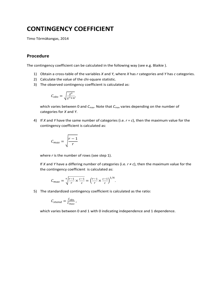
CONTINGENCY COEFFICIENT
Timo Törmäkangas, 2014
Procedure
The contingency coefficient can be calculated in the following way (see e.g. Blaikie ).
1) Obtain a cross-table of the variables X and Y, where X has r categories and Y has c categories.
2) Calculate the value of the chi-square statistic.
3) The observed contingency coefficient is calculated as:
√
,
which varies between 0 and Cmax. Note that Cmax varies depending on the number of
categories for X and Y.
4) If X and Y have the same number of categories (i.e. r = c), then the maximum value for the
contingency coefficient is calculated as:
√
where r is the number of rows (see step 1).
If X and Y have a differing number of categories (i.e. r ≠ c), then the maximum value for the
the contingency coefficient is calculated as:
√
(
)
.
5) The standardized contingency coefficient is calculated as the ratio:
,
which varies between 0 and 1 with 0 indicating independence and 1 dependence.
Example
Here is a cross-table for gender (sex) and self-assessed economic situation (nc1049).
From the above table we find χ2=4.912 and sample size n = 340. Although the chi-square statistic is
not statistically significant (p = 0.086), we calculate the observed contingency coefficient as:
√
√
.
The table has two rows (r = 2) and three columns (c = 3), hence the maximum of contingency
coefficient for this table is:
(
) (
)
.
The standardized contingency coefficient is:
.
This indicates that the relationship is weak between the variables. We can report the result as
showing no statistically significant dependence between gender and self-assessed economic
situation (standardized C = 0.157, p = 0.086).
References
Blaikie, N. 2003. Analyzing Quantative Data. London: SAGE.