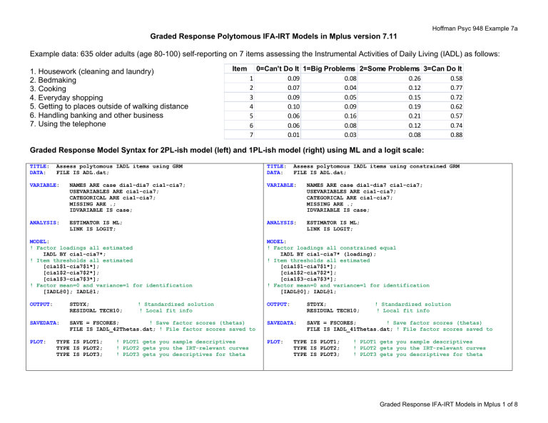
Hoffman Psyc 948 Example 7a
Graded Response Polytomous IFA-IRT Models in Mplus version 7.11
Example data: 635 older adults (age 80-100) self-reporting on 7 items assessing the Instrumental Activities of Daily Living (IADL) as follows:
1. Housework (cleaning and laundry)
2. Bedmaking
3. Cooking
4. Everyday shopping
5. Getting to places outside of walking distance
6. Handling banking and other business
7. Using the telephone
Item
1
2
3
4
5
6
7
0=Can't Do It 1=Big Problems 2=Some Problems 3=Can Do It
0.09
0.08
0.26
0.58
0.07
0.04
0.12
0.77
0.09
0.05
0.15
0.72
0.10
0.09
0.19
0.62
0.06
0.16
0.21
0.57
0.06
0.08
0.12
0.74
0.01
0.03
0.08
0.88
Graded Response Model Syntax for 2PL-ish model (left) and 1PL-ish model (right) using ML and a logit scale:
TITLE:
DATA:
Assess polytomous IADL items using GRM
FILE IS ADL.dat;
TITLE:
DATA:
Assess polytomous IADL items using constrained GRM
FILE IS ADL.dat;
VARIABLE:
NAMES ARE case dia1-dia7 cia1-cia7;
USEVARIABLES ARE cia1-cia7;
CATEGORICAL ARE cia1-cia7;
MISSING ARE .;
IDVARIABLE IS case;
VARIABLE:
NAMES ARE case dia1-dia7 cia1-cia7;
USEVARIABLES ARE cia1-cia7;
CATEGORICAL ARE cia1-cia7;
MISSING ARE .;
IDVARIABLE IS case;
ANALYSIS:
ESTIMATOR IS ML;
LINK IS LOGIT;
ANALYSIS:
ESTIMATOR IS ML;
LINK IS LOGIT;
MODEL:
! Factor loadings all estimated
IADL BY cia1-cia7*;
! Item thresholds all estimated
[cia1$1-cia7$1*];
[cia1$2-cia7$2*];
[cia1$3-cia7$3*];
! Factor mean=0 and variance=1 for identification
[IADL@0]; IADL@1;
MODEL:
! Factor loadings all constrained equal
IADL BY cia1-cia7* (loading);
! Item thresholds all estimated
[cia1$1-cia7$1*];
[cia1$2-cia7$2*];
[cia1$3-cia7$3*];
! Factor mean=0 and variance=1 for identification
[IADL@0]; IADL@1;
OUTPUT:
STDYX;
RESIDUAL TECH10;
OUTPUT:
STDYX;
RESIDUAL TECH10;
SAVEDATA:
SAVE = FSCORES;
! Save factor scores (thetas)
FILE IS IADL_42Thetas.dat; ! File factor scores saved to
SAVEDATA:
SAVE = FSCORES;
! Save factor scores (thetas)
FILE IS IADL_41Thetas.dat; ! File factor scores saved to
PLOT:
TYPE IS PLOT1;
TYPE IS PLOT2;
TYPE IS PLOT3;
! Standardized solution
! Local fit info
! PLOT1 gets you sample descriptives
! PLOT2 gets you the IRT-relevant curves
! PLOT3 gets you descriptives for theta
PLOT:
TYPE IS PLOT1;
TYPE IS PLOT2;
TYPE IS PLOT3;
! Standardized solution
! Local fit info
! PLOT1 gets you sample descriptives
! PLOT2 gets you the IRT-relevant curves
! PLOT3 gets you descriptives for theta
Graded Response IFA-IRT Models in Mplus 1 of 8
Hoffman Psyc 948 Example 7a
Graded Response Model 2PL-ish Model Fit (left) and 1PLish Model Fit (right) using ML logit:
MODEL FIT INFORMATION
MODEL FIT INFORMATION
Number of Free Parameters
28
Loglikelihood
H0 Value
-2523.585
Information Criteria
Akaike (AIC)
Bayesian (BIC)
Sample-Size Adjusted BIC
(n* = (n + 2) / 24)
5103.171
5227.828
5138.931
Chi-Square Test of Model Fit for the Binary and Ordered Categorical
(Ordinal) Outcomes**
Pearson Chi-Square
Value
Degrees of Freedom
P-Value
Number of Free Parameters
Loglikelihood
H0 Value
5226.620
5324.565
5254.717
Chi-Square Test of Model Fit for the Binary and Ordered Categorical
(Ordinal) Outcomes**
Pearson Chi-Square
Value
Degrees of Freedom
P-Value
2650.119
16321
1.0000
Likelihood Ratio Chi-Square
Value
Degrees of Freedom
P-Value
676.937
16317
1.0000
** Of the 48600 cells in the latent class indicator table, 38
were deleted in the calculation of chi-square due to extreme values.
-2591.310
Information Criteria
Akaike (AIC)
Bayesian (BIC)
Sample-Size Adjusted BIC
(n* = (n + 2) / 24)
1876.488
16317
1.0000
Likelihood Ratio Chi-Square
Value
Degrees of Freedom
P-Value
22
803.028
16321
1.0000
** Of the 48600 cells in the latent class indicator table, 40
were deleted in the calculation of chi-square due to extreme values.
This error message indicates that these 2 sets of chi-squares are not
on the same scale. We need to test the -2LL difference instead.
Does the 2PL-ish version of the GRM fit better than the 1PL-ish version?
−2523.585*-2 = 5047.170
−2591.310*-2 = 5182.620
−2ΔLL = 135.45, df = 6, p < .0001
AIC and BIC are smaller for 2PL, too
Graded Response IFA-IRT Models in Mplus 2 of 8
Hoffman Psyc 948 Example 7a
3 differently scaled solutions from ML logit (2 given, 1 calculated in excel) – all provide the exact same predictions!
UNSTANDARDIZED MODEL RESULTS (IFA MODEL SOLUTION)
Estimate
S.E.
Est./S.E.
Two-Tailed
P-Value
FACTOR LOADINGS = CHANGE IN LOGIT(Y) PER UNIT CHANGE IN THETA
IADL
BY
CIA1
6.846
0.841
8.140
0.000
CIA2
5.200
0.555
9.363
0.000
CIA3
4.613
0.456
10.119
0.000
CIA4
5.701
0.612
9.312
0.000
CIA5
3.556
0.298
11.950
0.000
CIA6
2.897
0.261
11.094
0.000
CIA7
1.778
0.209
8.512
0.000
THRESHOLDS = EXPECTED LOGIT(Y=0) WHEN THETA IS 0 (MEAN OF SAMPLE)
CIA1$1
-9.808
1.138
-8.620
0.000
CIA1$2
-6.460
0.799
-8.088
0.000
CIA1$3
-1.238
0.384
-3.226
0.001
CIA2$1
-8.145
0.794
-10.257
0.000
CIA2$2
-6.313
0.618
-10.219
0.000
CIA2$3
-3.737
0.441
-8.480
0.000
CIA3$1
-6.841
0.613
-11.162
0.000
CIA3$2
-5.194
0.480
-10.810
0.000
CIA3$3
-2.572
0.330
-7.792
0.000
CIA4$1
-7.454
0.747
-9.975
0.000
CIA4$2
-4.635
0.514
-9.026
0.000
CIA4$3
-1.426
0.327
-4.366
0.000
CIA5$1
-6.578
0.494
-13.314
0.000
CIA5$2
-3.041
0.273
-11.155
0.000
CIA5$3
-0.681
0.203
-3.354
0.001
CIA6$1
-5.538
0.411
-13.486
0.000
CIA6$2
-3.583
0.285
-12.554
0.000
CIA6$3
-2.044
0.219
-9.344
0.000
CIA7$1
-5.810
0.472
-12.315
0.000
CIA7$2
-4.398
0.322
-13.673
0.000
CIA7$3
-2.951
0.237
-12.457
0.000
STDYX MODEL RESULTS (IFA MODEL SOLUTION)
Estimate
S.E.
Est./S.E.
Two-Tailed
P-Value
FACTOR LOADINGS IN STANDARDIZED METRIC = loading*SD(Theta)/SD(Y)
IADL
BY
CIA1
0.967
0.008
124.093
0.000
CIA2
0.944
0.011
86.315
0.000
CIA3
0.931
0.012
75.583
0.000
CIA4
0.953
0.009
101.294
0.000
CIA5
0.891
0.015
57.872
0.000
CIA6
0.848
0.022
39.402
0.000
CIA7
0.700
0.042
16.689
0.000
(rest omitted)
USING RESULTS FROM IFA MODEL (LEFT PANEL):
IFA model: Logit(y=1) = –threshold + loading(Theta)
Threshold = expected logit of (y=0) for someone with Theta=0
When *-1, threshold becomes intercept: expected logit for (y=1) instead
Loading = regression of item logit on Theta
For 4-category responses, the sub-models look like this:
Logit(y= 0 vs 123) = -threshold$1 + loading(Theta)
Logit(y= 01 vs 23) = -threshold$2 + loading(Theta)
Logit(y= 012 vs 3) = -threshold$3 + loading(Theta)
IFA Models:
$1 Logit(CIA1=0 vs 123)= 9.808 + 6.846(Theta)  if Theta=0, prob=.99994
$2 Logit(CIA1=01 vs 23)= 6.460 + 6.846(Theta)  if Theta=0, prob=.99844
$3 Logit(CIA1=012 vs 3)= 1.238 + 6.846(Theta)  if Theta=0, prob=.77522
$1  if Theta=-1, logit= 2.962, prob= .95083
$2  if Theta=-1, logit= -0.386, prob= .40468
$3  if Theta=-1, logit= -5.608 prob= .00365
RESULTS FROM IRT MODEL MUST BE CALCULATED BY YOU!
IRT model: Logit(y) = a(theta – difficulty)
a = discrimination (rescaled slope) = loading
b = difficulty (location on latent metric) = threshold/loading
My calculations (see spreadsheet):
CIA1 loading = 6.846  a discrimination = 6.846
CIA1 threshold$1 = -9.808/6.846  b difficulty$1 = -1.433
CIA1 threshold$2 = -6.460/6.846  b difficulty$2 = -0.944
CIA1 threshold$3 = -1.238/6.846  b difficulty$3 = -0.181
For 4-category responses, the sub-models look like this:
$1 Logit(y= 0 vs 123) = a(theta – difficulty$1)
$2 Logit(y= 01 vs 23) = a(theta – difficulty$2)
$3 Logit(y= 012 vs 3) = a(theta – difficulty$3)
IRT Models:
$1 Logit = 6.846(Theta - -1.433)
$2 Logit = 6.846(Theta - -0.944)
$3 Logit = 6.846(Theta - -0.181)
Graded Response IFA-IRT Models in Mplus 3 of 8
Hoffman Psyc 948 Example 7a
Mplus Category Response Curves – Item 1 (good and steep discrimination) and Item 7 (less good because less steep)
Test Information
28
24
20
Theta Standard Error
The test has NO
information at all
past Theta = 1!
16
12
Info 4 =
Reliability .80
8
4
0
‐3.0
‐2.4
‐1.8 ‐1.2 ‐0.6 0.0 0.6 1.2
Theta (Mean = 0, Variance = 1)
1.8
Theta Standard Error
Test Information
Info 30 =
Reliability .97
2.0
1.8
1.6
1.4
1.2
1.0
0.8
0.6
0.4
0.2
0.0
SE = 1 /SQRT(info)
‐3.0 ‐2.4 ‐1.8 ‐1.2 ‐0.6 0.0 0.6 1.2 1.8
Theta (Mean = 0, Variance = 1)
Graded Response IFA-IRT Models in Mplus 4 of 8
Hoffman Psyc 948 Example 7a
Distribution of Theta under GRM (made in Mplus)
Although reliability is above .80 from about −2.0 to 0.4 or so, we still see a huge ceiling effect –
most of our sample can do all the tasks. If we are concerned about measuring the higher end of
theta better, then we’d need additional more difficult items for sure!
SAMPLE STATISTICS FOR
ESTIMATED FACTOR SCORES
1
SAMPLE STATISTICS
Means
IADL
IADL_SE
________
________
-0.018
0.394
Covariances
IADL
________
IADL
0.803
IADL_SE
0.140
IADL_SE
________
0.042
01 vs 23
012 vs 3
1.00
Item Difficulty
‐1.0
‐1.5
‐2.0
‐2.5
‐3.0
‐3.5
Probability of y = 1 if Theta = 0
0.0
‐0.5
Below is the probability of y=1 for each submodel if
Theta=0, as calculated from the thresholds as
1 – [exp(threshold) / (1+(exp(threshold))]
Only the last distinction of “can do it” has any items with
a chance of failure, so these items are very easy for a
person with average ability.
Variability in Spread of Item Difficulty (made in excel):
Some items (like 5) have a wider spread of their category thresholds,
but all categories appear useful (differentiable).
0 vs 123
The estimated theta scores are supposed to have a mean
of 0 and a variance of 1, but this table shows they have a
variance of only .803 instead. Such shrinkage is why it can
be problematic to use these estimated theta scores as
observed variables in other analyses.
0 vs 123
01 vs 23
012 vs 3
0.95
0.90
0.85
0.80
0.75
0.70
0.65
0.60
Graded Response IFA-IRT Models in Mplus 5 of 8
Hoffman Psyc 948 Example 7a
Here is the graded response model again: a 2PL-ish version vs. a 1PL-ish for Polytomous Responses using WLSMV probit model
TITLE: 2PL Graded Response Model under WLSMV
DATA:
FILE IS ADL.dat;
VARIABLE:
NAMES ARE case dia1-dia7 cia1-cia7;
USEVARIABLES ARE cia1-cia7;
CATEGORICAL ARE cia1-cia7;
MISSING ARE .;
IDVARIABLE IS case;
TITLE: 1PL Graded Response Model under WLSMV
DATA:
FILE IS ADL.dat;
VARIABLE:
NAMES ARE case dia1-dia7 cia1-cia7;
USEVARIABLES ARE cia1-cia7;
CATEGORICAL ARE cia1-cia7;
MISSING ARE .;
IDVARIABLE IS case;
ANALYSIS:
ANALYSIS:
ESTIMATOR IS WLSMV; PARAMETERIZATION IS THETA;
ESTIMATOR IS WLSMV; PARAMETERIZATION IS THETA;
DIFFTEST=2PL.dat; ! Use saved info from bigger model
MODEL:
! Factor loadings all estimated in 2PL
IADL BY cia1-cia7*;
! Item thresholds all estimated
[cia1$1-cia7$1*];
[cia1$2-cia7$2*];
[cia1$3-cia7$3*];
! Factor mean=0 and variance=1 for identification
[IADL@0]; IADL@1;
MODEL:
! Factor loadings all constrained equal in 1PL
IADL BY cia1-cia7* (loading);
! Item thresholds all estimated
[cia1$1-cia7$1*];
[cia1$2-cia7$2*];
[cia1$3-cia7$3*];
! Factor mean=0 and variance=1 for identification
[IADL@0]; IADL@1;
OUTPUT:
SAVEDATA:
OUTPUT:
SAVEDATA:
PLOT:
STDYX Residual;
! Standardized solution, local fit
DIFFTEST=2PL.dat; ! Save info from bigger model
SAVE = FSCORES;
! Save factor scores (thetas)
FILE IS IADL_42Thetas.dat; ! File factor scores saved to
TYPE IS PLOT1 PLOT2 PLOT3;
! Get IRT plots
MODEL FIT INFORMATION
Number of Free Parameters
Chi-Square Test of Model Fit
Value
Degrees of Freedom
P-Value
! Standardized solution, local fit
SAVE = FSCORES;
! Save factor scores (thetas)
FILE IS IADL_41Thetas.dat; ! File factor scores saved to
PLOT:
TYPE IS PLOT1 PLOT2 PLOT3;
! Get IRT plots
MODEL FIT INFORMATION
Number of Free Parameters
28
CFI/TLI
0.997
0.995
Chi-Square Test of Model Fit for the Baseline Model
Value
26556.135
Degrees of Freedom
21
P-Value
0.0000
22
Chi-Square Test of Model Fit
Value
Degrees of Freedom
P-Value
96.262*
14
0.0000
RMSEA (Root Mean Square Error Of Approximation)
Estimate
0.096
90 Percent C.I.
0.079
Probability RMSEA <= .05
0.000
CFI
TLI
STDYX Residual;
0.115
202.569*
20
0.0000
Chi-Square Test for Difference Testing
Value
Degrees of Freedom
P-Value
93.833
6
0.0000
RMSEA (Root Mean Square Error Of Approximation)
Estimate
0.120
90 Percent C.I.
0.105
Probability RMSEA <= .05
0.000
0.135
CFI/TLI
CFI
TLI
0.993
0.993
The Chi-Square for Difference Testing tells us directly that the 2PL
version of the polytomous model fits significantly better
(now under WLSMV, same as it did under ML).
Graded Response IFA-IRT Models in Mplus 6 of 8
Hoffman Psyc 948 Example 7a
Here are the parameter estimates under WLSMV Theta Parameterization (Probit) for the 2PL version of polytomous responses
UNSTANDARDIZED MODEL RESULTS (IFA MODEL SOLUTION)
Estimate
S.E.
Est./S.E.
Two-Tailed
P-Value
FACTOR LOADINGS = CHANGE IN PROBIT(Y=1) PER UNIT CHANGE
IADL
BY
CIA1
3.655
0.330
11.083
CIA2
3.346
0.388
8.632
CIA3
2.923
0.269
10.881
CIA4
3.286
0.299
11.008
CIA5
2.222
0.159
13.963
CIA6
1.907
0.169
11.305
CIA7
1.075
0.130
8.279
THRESHOLDS = EXPECTED PROBIT(Y=0)
CIA1$1
-5.151
CIA1$2
-3.658
CIA1$3
-0.734
CIA2$1
-5.096
CIA2$2
-4.253
CIA2$3
-2.620
CIA3$1
-4.193
CIA3$2
-3.404
CIA3$3
-1.761
CIA4$1
-4.379
CIA4$2
-2.987
CIA4$3
-1.024
CIA5$1
-3.866
CIA5$2
-1.892
CIA5$3
-0.425
CIA6$1
-3.450
CIA6$2
-2.354
CIA6$3
-1.400
CIA7$1
-3.282
CIA7$2
-2.577
CIA7$3
-1.757
WHEN THETA IS 0
0.424
-12.137
0.347
-10.534
0.217
-3.383
0.497
-10.254
0.445
-9.552
0.353
-7.425
0.327
-12.825
0.296
-11.486
0.232
-7.592
0.342
-12.794
0.269
-11.107
0.211
-4.863
0.233
-16.616
0.160
-11.856
0.130
-3.277
0.235
-14.697
0.184
-12.805
0.154
-9.072
0.249
-13.169
0.181
-14.231
0.137
-12.840
IN THETA
0.000
0.000
0.000
0.000
0.000
0.000
0.000
0.000
0.000
0.001
0.000
0.000
0.000
0.000
0.000
0.000
0.000
0.000
0.000
0.000
0.000
0.001
0.000
0.000
0.000
0.000
0.000
0.000
STDYX MODEL RESULTS (STANDARDIZED IFA MODEL SOLUTION)
FACTOR LOADINGS IN STANDARDIZED METRIC = loading*SD(Theta)/SD(Y)
IADL
BY
CIA1
0.965
0.006
159.169
0.000
CIA2
0.958
0.009
105.293
0.000
CIA3
0.946
0.009
103.821
0.000
CIA4
0.957
0.007
129.875
0.000
CIA5
0.912
0.011
82.875
0.000
CIA6
0.886
0.017
52.429
0.000
CIA7
0.732
0.041
17.844
0.000
Logit = 1.7*probit, or Probit = Logit/1.7
IFA model: Probit(y=1) = –threshold + loading(Theta)
Threshold = expected probit of (y=0) for someone with Theta=0
When *-1, threshold  intercept: expected probit for (y=1) instead
Loading = regression of item probit on Theta
For 4-category responses, the sub-models look like this:
Probit(y= 0 vs 123) = -threshold$1 + loading(Theta)
Probit(y= 01 vs 23) = -threshold$2 + loading(Theta)
Probit y= 012 vs 3) = -threshold$3 + loading(Theta)
IRT RESULTS ARE NOT GIVEN FOR POLYTOMOUS ITEMS;
THEY MUST BE CALCULATED BY YOU!
IRT model: Probit(y) = a(theta – difficulty)
a = discrimination (rescaled slope) = loading
b = difficulty (location on latent metric) = threshold/loading
For 4-category responses, the sub-models look like this:
$1 Probit(y= 0 vs 123) = a(theta – difficulty$1)
$2 Probit(y= 01 vs 23) = a(theta – difficulty$2)
$3 Probit(y= 012 vs 3) = a(theta – difficulty$3)
LOCAL FIT VIA STANDARDIZED RESIDUAL CORRELATIONS
LEFTOVER POLYCHORIC CORRELATION (HOW FAR OFF FROM DATA)
Residuals for Covariances/Correlations/Residual Correlations
CIA1
CIA2
CIA3
CIA4
CIA5
CIA6
_______ _______ ________ _______ _______ _______
CIA1
CIA2
0.013
CIA3
0.012
0.017
CIA4 -0.010
-0.025
-0.036
CIA5 -0.030
-0.045
-0.067
0.032
CIA6 -0.040
-0.055
-0.025
0.026
0.035
CIA7 -0.026
-0.007
0.016
0.022
-0.031
0.025
Graded Response IFA-IRT Models in Mplus 7 of 8
Hoffman Psyc 948 Example 7a
Bonus material! Here is how to fit the modified graded response model in Mplus using ML. The item location is set as threshold 3, and
two distance parameters (c1 and c2) are held equal across items, so that the spread of the category thresholds is held equal.
TITLE:
DATA:
VARIABLE:
2PL MODIFIED Graded Response Model using ML
FILE IS ADL.dat;
NAMES ARE case dia1-dia7 cia1-cia7;
USEVARIABLES ARE cia1-cia7;
CATEGORICAL ARE cia1-cia7;
MISSING ARE .;
IDVARIABLE IS case;
ANALYSIS:
OUTPUT:
SAVEDATA:
ESTIMATOR IS ML; LINK IS LOGIT;
STDYX TECH10;
! Standardized solution, local fit
SAVE = FSCORES;
! Save factor scores (thetas)
FILE IS MGRM_Thetas.dat; ! File factor scores saved to
TYPE IS PLOT1 PLOT2 PLOT3;
! Get IRT plots
PLOT:
MODEL:
! Threshold 1 is location - c1 as defined in NEW
[cia1$1] (t11);
[cia2$1] (t12);
[cia3$1] (t13);
[cia4$1] (t14);
[cia5$1] (t15);
[cia6$1] (t16);
[cia7$1] (t17);
! Threshold 2 is location - c2 as defined in NEW
[cia1$2] (t21);
[cia2$2] (t22);
[cia3$2] (t23);
[cia4$2] (t24);
[cia5$2] (t25);
[cia6$2] (t26);
[cia7$2] (t27);
! Threshold 3 defines location per item
[cia1$3] (loc1);
[cia2$3] (loc2);
[cia3$3] (loc3);
[cia4$3] (loc4);
[cia5$3] (loc5);
[cia6$3] (loc6);
[cia7$3] (loc7);
! Factor variance fixed to 1, mean fixed to 0 for identification
IADL@1; [IADL@0];
MODEL CONSTRAINT:
NEW(c1 c2);
! New category spread parameters
! Threshold 1 is location - c1 as defined in NEW
t11 = loc1 - c1;
t12 = loc2 - c1;
t13 = loc3 - c1;
t14 = loc4 - c1;
t15 = loc5 - c1;
t16 = loc6 - c1;
t17 = loc7 - c1;
! Threshold 2 is location – c2 as defined in NEW
t21 = loc1 - c2;
t22 = loc2 - c2;
Relative to the original graded response model,
t23 = loc3 - c2;
this modified model fits significantly worse,
t24 = loc4 - c2;
−2ΔLL(12) = 127, p < .001. However, we could
t25 = loc5 - c2;
examine for which items these constraints do not
t26 = loc6 - c2;
hold and free just those, resulting a hybrid or
t27 = loc7 - c2;
“partially modified” graded response model.
MODEL FIT INFORMATION
Number of Free Parameters
Loglikelihood
H0 Value
Information Criteria
Akaike (AIC)
Bayesian (BIC)
Sample-Size Adjusted BIC
(n* = (n + 2) / 24)
MODEL RESULTS
Estimate
IADL
BY
CIA1
4.195
CIA2
5.507
CIA3
5.025
CIA4
4.943
CIA5
3.238
CIA6
3.725
CIA7
2.169
Means
IADL
0.000
Thresholds
CIA1$1
-5.971
CIA1$2
-3.569
CIA1$3
-1.079
CIA2$1
-8.729
CIA2$2
-6.327
CIA2$3
-3.838
CIA3$1
-7.615
CIA3$2
-5.213
CIA3$3
-2.723
CIA4$1
-6.235
CIA4$2
-3.833
CIA4$3
-1.344
CIA5$1
-5.463
CIA5$2
-3.061
CIA5$3
-0.571
CIA6$1
-7.084
CIA6$2
-4.682
CIA6$3
-2.192
CIA7$1
-8.004
CIA7$2
-5.602
CIA7$3
-3.113
Variances
IADL
1.000
New/Additional Parameters
C1
4.891
C2
2.489
16
-2586.984
5205.968
5277.201
5226.403
S.E.
Est./S.E.
Two-Tailed
P-Value
0.291
0.433
0.379
0.362
0.212
0.274
0.240
14.439
12.711
13.249
13.645
15.254
13.607
9.054
0.000
0.000
0.000
0.000
0.000
0.000
0.000
0.000
999.000
999.000
0.293
0.255
0.240
0.455
0.431
0.414
0.384
0.354
0.338
0.332
0.296
0.282
0.244
0.202
0.185
0.311
0.277
0.256
0.314
0.285
0.265
-20.350
-13.993
-4.492
-19.197
-14.676
-9.270
-19.816
-14.738
-8.065
-18.801
-12.945
-4.765
-22.411
-15.184
-3.089
-22.756
-16.906
-8.557
-25.509
-19.660
-11.734
0.000
0.000
0.000
0.000
0.000
0.000
0.000
0.000
0.000
0.000
0.000
0.000
0.000
0.000
0.002
0.000
0.000
0.000
0.000
0.000
0.000
0.000
999.000
999.000
0.167
0.095
29.309
26.316
0.000
0.000
Graded Response IFA-IRT Models in Mplus 8 of 8