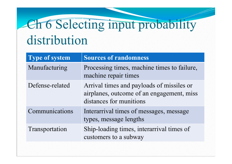
Ch 6 Selecting input probability
distribution
Type of system
Manufacturing
Defense-related
Sources of randomness
Processing times, machine times to failure,
machine repair times
Arrival times and payloads of missiles or
airplanes, outcome of an engagement, miss
distances for munitions
Communications
Interarrival times of messages, message
types, message lengths
Transportation
Ship-loading times, interarrival times of
customers to a subway
y A single-server queueing system has exponential
interarrival times with a mean of 1 minute. Suppose that
200 service times are available from the system, but their
underlying probability distribution is unknown.
Service-time
distribution
Average delay in
queue
Average number
in queue
Proportion of
delays ≧20
Exponential
6.71
6.78
0.064
Gamma
4.54
4.6
0.019
Weibull
4.36
4.41
0.013
Logormal
7.19
7.3
0.078
Normal
6.04
6.13
0.045
Specify a distribution
y Approach 1: the data values themselves are used directly
in the simulation
y Approach 2: the data values themselves are used an
empirical distribution function
y Approach 3: standard techniques of statistical inference
are used to “fit” a theoretical distribution form to the data
and to perform hypothesis tests to determine the goodness
of fit
y Drawback of approach 1
y The simulation can only reproduce what has happened
historically
y There is seldom enough data to make all the desired
simulation runs
y Approach 2 avoids these shortcomings (for continuous
data)
y If a theoretical distribution can be found that fits the observed
data reasonably well, then this will generally be preferable to
using an empirical distribution for the following reasons:
y An empirical distribution function may have certain
“irregularities,” particularly if only a small number of data values
are available
y If empirical distributions are used in the usual way, it is not
possible to generate values outside the range of the observed data
in the simulation
y There may be a compelling physical reason in some situations for
using a certain theoretical distribution form as a model for a
particular input random variable.
y A theoretical distribution is a compact way of representing a set
of data values.
y A theoretical distribution is easier to change.
6.2 Useful probability distribution
y The purpose is to discuss a variety of distribution that
have been found to be useful in simulation modeling and
to provide a unified listing of relevant properties of these
distributions.
y Continuous distribution (CD)
y Discrete distribution (DD)
6.2.1 Parameterization of CD
y Three types of parameters
y Location parameter γ specifies an abscissa (x axis)
location point of a distribution’s range of values. (usually γ
is the midpoint or lower endpoint of the distribution’s range)
y Y=X+ γ
y Scale parameter β determines the scale (or unit) of
measurement of the values in the range of the distribution.
y Y= β X
y Shape parameter α determines, distinct from location and
scale, the basic form or shape of a distribution within the
general family of distributions of interest.
6.2.2 Continuous distribution
y Uniform
y Exponential
y Gamma
y Weibull
y Normal
y Longormal
y Beta
y Pearson type V, VI
y Log-logistic
y Johnson SB , SU
y Triangular
Discrete distribution
y
y
y
y
y
y
Bernoulli
Discrete uniform
Binomial
Geometric
Negative binormal
Poisson
6.3 Techniques for assessing
sample independence