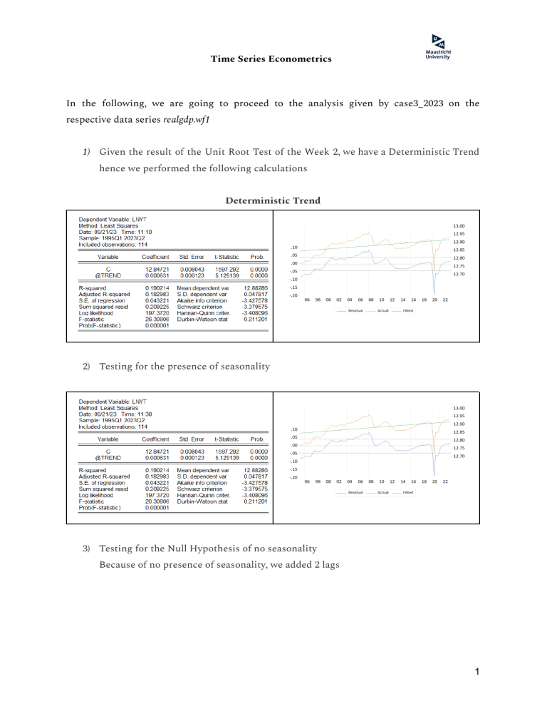
Time Series Econometrics
In the following, we are going to proceed to the analysis given by case3_2023 on the
respective data series realgdp.wf1
1) Given the result of the Unit Root Test of the Week 2, we have a Deterministic Trend
hence we performed the following calculations
Deterministic Trend
2) Testing for the presence of seasonality
3) Testing for the Null Hypothesis of no seasonality
Because of no presence of seasonality, we added 2 lags
1
Week 1 - Time Series Econometrics
4) Why is that so?
The overall F-statistic of a trend stationary model evaluates the overall significance
of the entire model including the joint insignificance of your intercept in its null
hypothesis while the Wald F-statistic test does not.
5) Given our LM Test = 0.21, we have the presence of autocorrelation hence we perform
the F-test after having robustified the standard error and there’s no autocorrelation
anymore because of the White Test, we accept the Null = 1.319 and hence there’s
Homoskedasticity
2
Week 1 - Time Series Econometrics
6) Test for autocorrelation -
Our best model is Log(RealGDP) with 2 lags
7)
3
Week 1 - Time Series Econometrics
8) Test for the presence of a break at some chosen date
9) Test for the presence of one endogenous break
10) Test for the presence of several endogenous break
Germany(-1)
4
Week 1 - Time Series Econometrics
11) White and Q for New Model
White
Q
12) Reestimate your equation without the last 10 (because last 2 are within the break)
observations and compute RMSE for dynamic and static forecast
Static
Dynamic
5
Week 1 - Time Series Econometrics
13) Diebold Mariano Test
14) No strong seasonal pattern
6