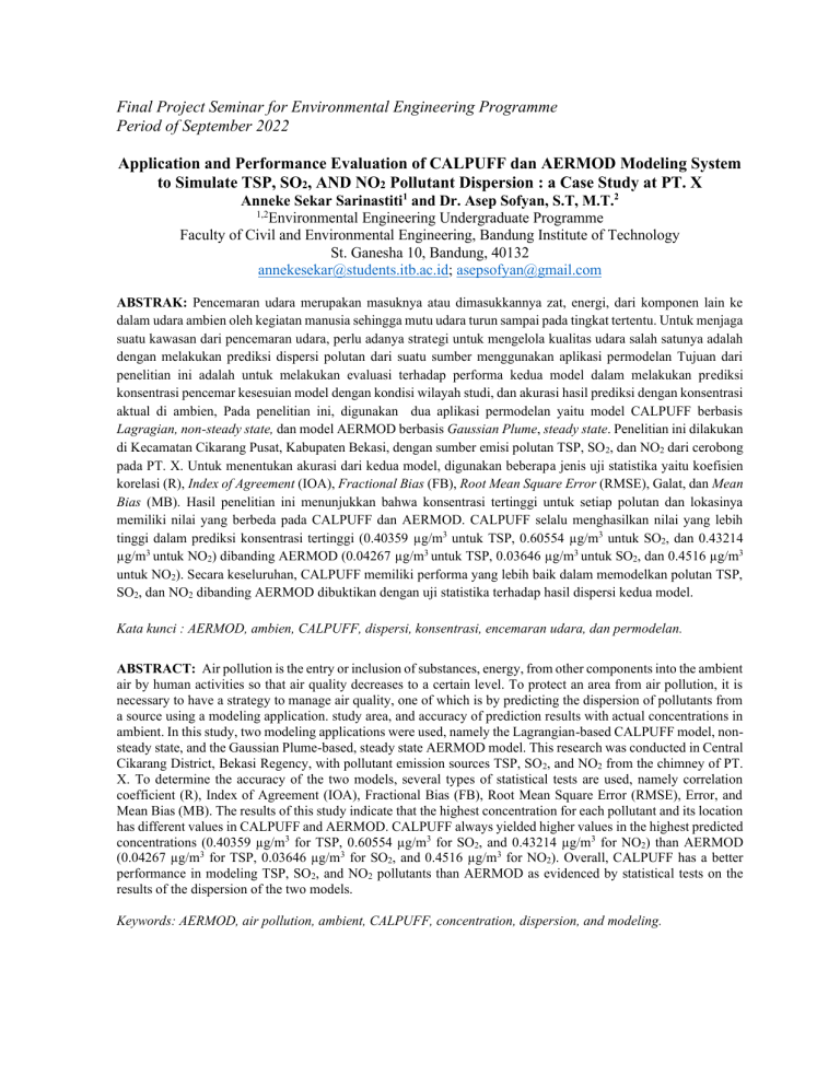
Final Project Seminar for Environmental Engineering Programme
Period of September 2022
Application and Performance Evaluation of CALPUFF dan AERMOD Modeling System
to Simulate TSP, SO2, AND NO2 Pollutant Dispersion : a Case Study at PT. X
Anneke Sekar Sarinastiti1 and Dr. Asep Sofyan, S.T, M.T.2
1,2
Environmental Engineering Undergraduate Programme
Faculty of Civil and Environmental Engineering, Bandung Institute of Technology
St. Ganesha 10, Bandung, 40132
annekesekar@students.itb.ac.id; asepsofyan@gmail.com
ABSTRAK: Pencemaran udara merupakan masuknya atau dimasukkannya zat, energi, dari komponen lain ke
dalam udara ambien oleh kegiatan manusia sehingga mutu udara turun sampai pada tingkat tertentu. Untuk menjaga
suatu kawasan dari pencemaran udara, perlu adanya strategi untuk mengelola kualitas udara salah satunya adalah
dengan melakukan prediksi dispersi polutan dari suatu sumber menggunakan aplikasi permodelan Tujuan dari
penelitian ini adalah untuk melakukan evaluasi terhadap performa kedua model dalam melakukan prediksi
konsentrasi pencemar kesesuian model dengan kondisi wilayah studi, dan akurasi hasil prediksi dengan konsentrasi
aktual di ambien, Pada penelitian ini, digunakan dua aplikasi permodelan yaitu model CALPUFF berbasis
Lagragian, non-steady state, dan model AERMOD berbasis Gaussian Plume, steady state. Penelitian ini dilakukan
di Kecamatan Cikarang Pusat, Kabupaten Bekasi, dengan sumber emisi polutan TSP, SO 2, dan NO2 dari cerobong
pada PT. X. Untuk menentukan akurasi dari kedua model, digunakan beberapa jenis uji statistika yaitu koefisien
korelasi (R), Index of Agreement (IOA), Fractional Bias (FB), Root Mean Square Error (RMSE), Galat, dan Mean
Bias (MB). Hasil penelitian ini menunjukkan bahwa konsentrasi tertinggi untuk setiap polutan dan lokasinya
memiliki nilai yang berbeda pada CALPUFF dan AERMOD. CALPUFF selalu menghasilkan nilai yang lebih
tinggi dalam prediksi konsentrasi tertinggi (0.40359 µg/m3 untuk TSP, 0.60554 µg/m3 untuk SO2, dan 0.43214
µg/m3 untuk NO2) dibanding AERMOD (0.04267 µg/m3 untuk TSP, 0.03646 µg/m3 untuk SO2, dan 0.4516 µg/m3
untuk NO2). Secara keseluruhan, CALPUFF memiliki performa yang lebih baik dalam memodelkan polutan TSP,
SO2, dan NO2 dibanding AERMOD dibuktikan dengan uji statistika terhadap hasil dispersi kedua model.
Kata kunci : AERMOD, ambien, CALPUFF, dispersi, konsentrasi, encemaran udara, dan permodelan.
ABSTRACT: Air pollution is the entry or inclusion of substances, energy, from other components into the ambient
air by human activities so that air quality decreases to a certain level. To protect an area from air pollution, it is
necessary to have a strategy to manage air quality, one of which is by predicting the dispersion of pollutants from
a source using a modeling application. study area, and accuracy of prediction results with actual concentrations in
ambient. In this study, two modeling applications were used, namely the Lagrangian-based CALPUFF model, nonsteady state, and the Gaussian Plume-based, steady state AERMOD model. This research was conducted in Central
Cikarang District, Bekasi Regency, with pollutant emission sources TSP, SO 2, and NO2 from the chimney of PT.
X. To determine the accuracy of the two models, several types of statistical tests are used, namely correlation
coefficient (R), Index of Agreement (IOA), Fractional Bias (FB), Root Mean Square Error (RMSE), Error, and
Mean Bias (MB). The results of this study indicate that the highest concentration for each pollutant and its location
has different values in CALPUFF and AERMOD. CALPUFF always yielded higher values in the highest predicted
concentrations (0.40359 µg/m3 for TSP, 0.60554 µg/m3 for SO2, and 0.43214 µg/m3 for NO2) than AERMOD
(0.04267 µg/m3 for TSP, 0.03646 µg/m3 for SO2, and 0.4516 µg/m3 for NO2). Overall, CALPUFF has a better
performance in modeling TSP, SO2, and NO2 pollutants than AERMOD as evidenced by statistical tests on the
results of the dispersion of the two models.
Keywords: AERMOD, air pollution, ambient, CALPUFF, concentration, dispersion, and modeling.
1.
INTRODUCTION
Air pollution is the entry or inclusion of substances, energy, from other components into ambient air by
human activities so that air quality drops to a certain level which causes ambient air to be unable to fulfill
its function (PP No. 41 of 1999 concerning Air Pollution Control). To protect an area from air pollution,
it is necessary to have a strategy to manage air quality. The air quality monitoring system is a strategy to
determine the level of pollution in an area and an action plan to implement policies and laws and
regulations for air quality management. In this strategy, a dispersion model is needed to determine the
pattern of pollutant distribution and also the maximum concentration as an effort to estimate or forecast
the impacts that can occur. There are two systems that can be used to model polluters, namely the
CALPUFF (California Puff) model and the AERMOD (The American Meteorology Society
Environmental Protection Agency Regulatory Model).
CALPUFF uses a non-steady state approach that takes into account the effects of spatial changes and
meteorological components and surface characteristics. AERMOD is a Gaussian plume model-based
software recommended by the US EPA for air quality simulation (EPA, 2005; Rood, 2014). AERMOD
uses a steady state approach that can include complete climate data such as the planetary boundary layer
(PBL).
PT. X is an automotive casting factory located in Central Cikarang, Bekasi Regency, West Java.
Production activities at PT.X include pressing, welding, painting, engine assembly, and aftersales. From
the production process, PT. X utilizes combustion or evaporation processes, the by-products of which
are released into the air which have the potential to cause air pollution. Therefore, it is necessary to model
the prediction of pollutant distribution in PT. X to determine the distribution of pollutants and determine
the comparison between the CALPUFF and AERMOD models. To determine the accuracy of the two
models, several types of statistical tests were used, namely correlation coefficient (R), Index of
Agreement (IOA), Fractional Bias (FB), Root Mean Square Error (RMSE), Error, and Mean Bias (MB).
2.
OBJECTIVE
The purpose of this study was to identify the sources of pollution in PT. X, predicting the distribution of
pollutants in PT. X using CALPUFF and AERMOD software, determine the comparison of the
distribution and the ability of the two applications in modeling, determine recommendations for using
the model according to the geographical and meteorological conditions of the research location.
3.
METHODOLOGY
3.1
Secondary Data Collection
Secondary data collection was carried out to assist authors in writing reports on the preparation of
technical approvals for emissions. Secondary data obtained from PT. X in the form of emission
concentration data at the chimney, ambient air data at PT. X. Table 3.1 shows the chimney data of PT.
X. and Table 3.2 shows emission data from PT. X.
Table 3.1 Chimney Data of PT. X
Tabel 3.2 Emission Data of PT. X
Other data that the author get are topography, land use data around PT. X, as well as surface and upper
air meteorological data in the area around PT. X. Topographic data is obtained through the website
www.src.com, meteorological data is obtained through the website www.copernicus.com, and land use
data is obtained from global land uses.
3.2
Calculation of Emission Rate
Determination of emission rate is an early stage before conducting modeling. Emission rate is an
important factor that affects the value and pattern of pollutant concentration produced
3.2.1 Calculation of Average Wind Speed
Before calculating the emission rate, it is necessary to calculate the peak speed of the chimney first,
which requires wind speed data from the research location. The average wind speed of the study area is
determined as follows:
𝑎𝑣𝑔 𝑤𝑖𝑛𝑑 𝑠𝑝𝑒𝑒𝑑
(𝑚𝑒𝑑𝑖𝑎𝑛 𝑣𝑎𝑙𝑢𝑒 1 𝑥 % 𝑜𝑓 𝑤𝑖𝑛𝑑 1) + (𝑚𝑒𝑑𝑖𝑎𝑛 𝑣𝑎𝑙𝑢𝑒 2 𝑥 % 𝑜𝑓 𝑤𝑖𝑛𝑑 2) + (𝑚𝑒𝑑𝑖𝑎𝑛 𝑣𝑎𝑙𝑢𝑒 2 𝑥 % 𝑜𝑓 𝑤𝑖𝑛𝑑)
=
% 𝑡𝑜𝑡𝑎𝑙 𝑤𝑖𝑛𝑑 𝑝𝑒𝑟𝑐𝑒𝑛𝑡𝑎𝑔𝑒𝑠
The average wind speed obtained is 4.52 m/s.
3.2.2 Calculation of Top Chimney Velocity and Emission Rate
Gaussian equations are used to determine stack peak velocity and emission rate. The chimney peak
velocity is obtained through the following equation.
𝑈2
𝑧2 𝑝
=( )
𝑈1
𝑧1
Based on the calculation, the peak velocity of the chimney is 4.77 m/s for scrubber, 4.1 m/s for Dust
Collector 1, and 4.61 um/s for Dust Collector 2. Emission rate of each stacks can be calculated after
getting the top speed at each stack, through the following equation.
𝐸𝑚𝑖𝑠𝑠𝑖𝑜𝑛 𝑟𝑎𝑡𝑒 =
𝐶
1
2
4×𝜋×𝑑 ×𝑣
Based on the calculation, the velocity at each stack is 2.44 mg/s, 0.38 mg/s, and 0.29 mg/s at the scrubber
stack, 0.73 mg/s, 1.89 mg/s, and 1.54 mg/s at dust collector stack 1, and 0.55 mg/s, 0.67 mg/s, and 0.53
mg/s at dust collector stack 2, for pollutants TSP, SO2, and NO2.
3.3
Determination of Study Area Grid
The study area grid determination is needed to limit the distance over which the pollutant will be
modeled. In this study, a grid of 120 km x 80 km was used with a length of 1 km for each grid.
3.4
Pollutant Dispersion Modeling Using CALPUFF dan AERMOD
The collected data was processed using the CALPUFF AERMOD modeling application. Table 3.6 shows
the differences in input data for CALPUFF and AERMOD.
Tabel 3.6 Differences in input data on CALPUFF and AERMOD
In general, the data entered into the two models have the same criteria so that the different variables are
only the result of the dispersion of the two models. The main difference in entering input data in both
models is that the user needs to prepare all input data in CALPUFF before the process continues to the
next processor, while empty input data in AERMOD can be overcome by using the menu to create and
generate the data. All missing data parameters can be automatically calculated on AERMOD. Another
difference lies in the technical input of data input. In CALPUFF, the user needs to do the processing in
stages because the output of the first stage is the input for the next stage. In AERMOD, the user can
choose which stage to do first. Therefore, using AERMOD is easier and faster than using CALPUFF.
4.
ANALYSIS AND DISCUSSION
4.1 Calculation Results
Table 4.1 shows the results of the emission dispersion of TSP, SO2, and NO2 and the maximum
concentration received by the receptor in the period of 1 and 24 hours.
Table 4.1 The results of the emission dispersion of TSP (left), SO2 (right), and NO2 (bottom) and the
maximum concentrations received by receptors on CALPUFF and AERMOD
Figure 4.1 shows the mapping of the final concentration and ambient concentration of each pollutant for
the CALPUFF and AERMOD models.
Final and Ambien Concentration of SO2
Final and Ambient Concentration of TSP
Concentration (µg/m3)
120
100
Concentration (µg/m3)
100
80
60
40
CALPUFF
20
AERMOD
Data Ambien
0
0
1
2
3
4
5
6
CALPUFF
80
AERMOD
Data Ambien
60
40
20
0
Sampling Point
0
1
Sampling
Point
2
3
4
5
6
Final and Ambient Concentration of NO2
Concentration (µg/m3)
70
60
CALPUFF
AERMOD
Data Ambien
50
40
30
20
10
0
0
1
2
3
4
5
6
Sampling Point
Figure 4.1 Graph mapping the final concentration and ambient pollutant concentrations of TSP (left),
SO2 (right), and NO2 (bottom) on the CALPUFF and AERMOD models
In Figure 4.1, it can be seen that all final concentrations of dispersion have values that are generally
smaller than the ambient data. This can be caused by the use of background concentration data that is not
in accordance with the actual background concentration. Due to the limited background concentration
data sources, the background concentration data used are not entirely correct at the monitoring location
used so that the values may differ from actual conditions. In addition, different actual background
concentration conditions may be caused by location, meteorological conditions, regional development
projections, topography, land use, emission sources, other pollutants in ambient air, and other factors
that have a direct influence on the final dispersion result. In addition, the existence of emission sources
other than PT. X as well as biogenic and natural emissions at the research site which are not considered
in the modeling can also cause dispersion results that are not in accordance with ambient conditions
(Kesarkar et al., 2007).
It is seen that the TSP concentration curve has the same pattern whereas the ambient air concentration
increases, the final dispersion concentration also increases. Likewise, when the ambient concentration
decreases, the final dispersion concentration also decreases. The same pattern also occurs in the SO 2
pollutant mapping curve. However, this pattern was not found in the NO2 pollutant curve. At monitoring
point 3 in Figure 4.1, there is an outlier where the final concentration of the dispersion decreases as the
concentration in the ambient air increases. This condition can be caused by several things such as
incomplete meteorological data at that point during monitoring time, or differences in background
concentration which causes the final dispersion results to have far differences. But overall, the CALPUFF
model is considered to still be able to predict well according to the pattern in the ambient air even though
the final concentration and dispersion have very large differences in value, CALPUFF and there are also
outliers in NO2 pollutants.
One of the causes of the deviation of the final concentration from the above data with ambient air is due
to the incompleteness of the emission source data (Im U., Yenigun O, 2005). A perfect modeling and
producing precise pollutant predictions according to ambient data depends on the accuracy of the
emission inventory data of the plant concerned and the level of precision of the meteorological and
topographical data at the study site.
Deviations that occur in the validation test of the Gauss model can be caused by the research location
having a complex topography while Gauss's ability is limited to uncomplicated terrain. This happens
because it has a Gaussian Plume base in steady state conditions so it does not consider changes in
meteorological and field conditions in units of space and time. As a result, the AERMOD model is not
suitable for use in research sites with complex terrain, changing meteorological conditions because the
results will have values that are far from the ambient data. This is in accordance with the terrain
conditions in Bekasi Regency which have different land heights with a range of 3-40 meters above sea
level so that the Bekasi Regency terrain becomes complex. (BPS Bekasi Regency, 2022). In particular,
Cikarang Sub-district in Bekasi Regency has a topography of 15-46 mdpl, so that the meteorological data
available under these conditions is highly variable. This condition explains the deviation of the final
concentration values in AERMOD and CALPUFF.
Meteorological conditions can also cause data deviation on AERMOD, where AERMOD cannot model
pollutants with wind speeds <1 m/s (Masuraha, 2006). Based on surface meteorological data, there are
winds with a speed of <1 ms which are called calm winds as much as 2% during the research period.
This condition can explain the deviations made by the AERMOD model in modeling the three types of
pollutants at PT. X.
4.2
Statistics Test
After that, several statistical tests were conducted to determine the error and accuracy of the two models
in predicting pollutant concentrations and determine which model is more accurate. The following is the
equation used in this study to perform statistical tests.
2
𝐼𝑂𝐴 = 1 −
∑𝑁
𝑖=1(𝐶𝑝𝑟𝑒𝑑,𝑖 − 𝐶𝑜𝑏𝑠,𝑖 )
∑𝑁
𝑖=1(|𝐶𝑝𝑟𝑒𝑑,𝑖
− 𝐶𝑎𝑣𝑔𝑜𝑏𝑠 | + |𝐶𝑜𝑏𝑠,𝑖 − 𝐶𝑎𝑣𝑔𝑜𝑏𝑠 |)
Ideal value = >0.5
𝑅=
∑𝑁
𝑖=1(𝐶𝑝𝑟𝑒𝑑,𝑖 − 𝐶𝑎𝑣𝑔𝑝𝑟𝑒𝑑 ) × (𝐶𝑜𝑏𝑠,𝑖 − 𝐶𝑎𝑣𝑔𝑜𝑏𝑠 )
2
𝑁
2
√∑𝑁
𝑖=1(𝐶𝑝𝑟𝑒𝑑,𝑖 − 𝐶𝑎𝑣𝑔𝑝𝑟𝑒𝑑 ) × ∑𝑖=1(𝐶𝑜𝑏𝑠,𝑖 − 𝐶𝑎𝑣𝑔𝑜𝑏𝑠 )
Ideal value = close to 1
𝐹𝐵 =
Ideal value = -0.7 to 0.7
2
2 (𝐶𝑎𝑣𝑔𝑜𝑏𝑠 − 𝐶𝑎𝑣𝑔𝑝𝑟𝑒𝑑 )
𝐶𝑎𝑣𝑔𝑝𝑟𝑒𝑑 + 𝐶𝑎𝑣𝑔𝑜𝑏𝑠
𝐸𝑟𝑟𝑜𝑟 = |
𝐶𝑜𝑏𝑠 − 𝐶𝑝𝑟𝑒𝑑
| × 100%
𝐶𝑜𝑏𝑠
𝑛
1
𝑅𝑀𝑆𝐸 = √ ∑ (𝐶𝑝𝑟𝑒𝑑 − 𝐶𝑜𝑏𝑠 )2
𝑛
𝑖=1
𝑛
1
𝑀𝐵 = ∑ (𝐶𝑝𝑟𝑒𝑑 − 𝐶𝑜𝑏𝑠 )
𝑛
𝑖=1
Data for statistical test is the final concentration of dispersion data by CALPUFF and AERMOD and
ambient air concentration. Statistical tests were carried out by comparing the final concentration of the
dispersion with the concentration in ambient air at the same coordinate point.
The statistical test shows that CALPUFF has a higher accuracy than AERMOD in predicting the
concentration for each pollutant, as evidenced by the statistical test value of CALPUFF which tends to
be higher than AERMOD.
5.
CONCLUSION
Based on the research conducted, it can be concluded as follows:
1. CALPUFF has a Lagrangian non-steady state basis while AERMOD has a Gasussian Plume steady
state basis so that the difference in the prediction results of concentrations in the air.
2. CALPUFF is able to model concentration predictions more accurately than AERMOD because
CALPUFF pays attention to the reaction of each particle after it is dispersed, takes into account variations
in meteorological and topographical conditions in the study area at the time of observation, is able to
make predictions at each point and at certain hours, and takes into account the presence of calm winds
at the time of observation.
3. The statistical test proves that CALPUFF has more capabilities than AERMOD because the test results
are higher than the AERMOD test results.
6.
REFERENCES
Assomadi, Abdu. 2016. Air Pollutant Dispersion Model. Surabaya: ITS Environmental Engineering
Study Program.
Ahrens, DC 2009. Essentials of Meteorology: An Invitation to the Atmosphere. USA: Bros.
Central Bureau of Statistics (BPS) Bekasi Regency. 2022. Bekasi Regency in Figures. Jakarta: Central
Bureau of Statistics
Engineering and Scientific Consulting. 2011. CALPUFF Modeling System Version 6 User
Instruction
Government Regulation Number 41 of 1999 on Air Pollution Control.
Government Regulation of the Republic of Indonesia Number 101 of 2014 concerning Management of
Hazardous and Toxic Waste.
Kesarkar et al. 2007. Weather Research and Forecasting Model with AERMOD for pollutant dispersion
modeling. A case study for PM10 dispersion over Pune, India. Atmospheric Environment.
DOI:10.1016/j.atmosenv.2017
Law of the Republic of Indonesia Number 32 of 2009 concerning Environmental Protection and
Management Life.
Law No. 23 of 1997 concerning Environmental Management.
Regulation of the State Minister of the Environment of the Republic of Indonesia Number 22 of
2021 concerning the Implementation of Environmental Protection and Management.
Masuraha and Anand. 2006. Evaluation of the AERMOD Model and Examination of Required Length of
Meteorological Data for Computing Concentrations in Urban Areas. University of Toledo :
2006.
Regulation of the State Minister of the Environment of the Republic of Indonesia Number 12 of 2010
concerning the Implementation of Air Pollution Control in Regions
Regulation of the State Minister for the Environment of the Republic of Indonesia Number 5 of 2021
concerning Procedures for Issuing Technical Approval and Operational Eligibility Letters for
Environmental Pollution Control.
Models.
Rodhe, H., Grandell, J. 1972. The removal time of aerosol particles from the atmosphere by precipitation
scavenging. USA: Tellus 24 442.
Rood, Arthur S. 2014. Performance Evaluation of AERMOD, CALPUFF, and Legacy Air Dispersion
Models
Using
the
Winter
Validation
Tracer
Study
Dataset.
https://doi.org/10.1016/j.atmosenv.2014.02.054.
United States Environmental Protection Agency. 2005. Air Quality Dispersion Modeling –
Alternative Models.